Shaymaa Abdulrasool Hameed![]() | Ansam Adil Mohammed
| Ansam Adil Mohammed![]() | Haider Fawzi Mahmood*
| Haider Fawzi Mahmood*![]()
© 2026 The authors. This article is published by IIETA and is licensed under the CC BY 4.0 license (http://creativecommons.org/licenses/by/4.0/).
OPEN ACCESS
The Musayyib power plant in Babylon, Iraq, includes 7X LM6000 units, providing a power amount of 1,280 MW. This study developed an integrated mathematical model to simulate vibration responses of the LM6000 gas turbines when they operate in the actual conditions at the site, which include high ambient temperature, a wide range of fuel quality, and on/off electrical load variations in the Iraqi Power System. The mathematical model is validated by the operational data collected from the accelerometers and the proximity probes installed on turbine units at the Musayyib plant. Based on the results, the model accurately predicted the vibration response with an average absolute percentage error of 5.8% for the synchronous components, 10.3% for the sub-synchronous components, with a correlation coefficient of 0.942. Sensitivity studies have revealed that the vibration magnitudes increase dramatically with an increase in ambient temperature, differences in fuel heat value, and bearing temperature differences, which emphasizes the importance of thermal factors in vibration magnification. This model can be effectively utilized to determine the critical speeds, safety margins, and vibration magnitudes, which would be beneficial for the implementation of condition-based maintenance strategies in gas turbine power stations in hot environments.
mathematical modeling, vibration prediction, LM6000 gas turbine, rotor dynamics, thermal effects, Iraqi power infrastructure
1.1 Background and significance
Due to rapid industrialization and burgeoning population, the energy consumption in the world has also increased, so that gas turbine power is now utilized more for this purpose. The Middle East enjoys the blessing of abundant natural gas resources and a rapidly increasing rate of electricity demand. A huge number of investments have been made in turbine-based gas technology in the Middle East over the past 40 years [1]. And as an abundant oil and natural gas producer, Iraq has built a number of thermal power plants to complement its energy grid—the Musayyib Thermal Power Plant being one of the most important in the region.
Vibrations, and the knowledge of them and their effect, play a decisive role in gas turbine reliability and availability. Unbalanced vibrations in rotary machines can lead to approaching catastrophic failures, unexpected stoppage of processes, and extensive financial damage [2]. Therefore, in the power generation sector, which is vital for grid stability, the need for accurate vibration prediction models is highly desirable. Turbine failure has larger economic implications than the cost of repairs, as it results in forgone income resulting from lower energy production, disruption penalties, and wear and tear on assets [3].
Modern research has emphasized that vibration is the primary diagnosing tool and the need for a condition-based maintenance strategy in GTOps [4]. However, traditional reactive maintenance methods are no longer satisfactory for today's power plants, where economic and environmental considerations demand high efficiency and minimal downtime. This evolution in maintenance philosophy has been made possible by the use of predictive models that are able to predict levels of vibration for various operating conditions.
1.2 Gas turbine technology and LM6000 specifications
The General Electric LM6000 Gas Turbine, a derivative of the CF6-80C2 aircraft engine, is an example of an evolution in technology. The LM6000, which was originally developed in the 1990s, is well-accepted in the power industry because of its high efficiency, low emissions, and operational flexibility [5]. The turbine is of a simple cycle two-shaft type, including a low pressure (LP) compressor, a high pressure (HP) compressor, a combustion chamber, an HP turbine, and an LP turbine.
The LM6000 has technical specifications that include 43 MW rated power output, 42% thermal efficiency, and a pressure ratio of 30:1 [6]. The turbine is rated at 3,600 RPM for 60 Hz service and is suitable for fast loading and frequent start-stop cycles. These features make the LM6000 ideal for peak power and grid support in emerging electricity markets.
The rotor dynamics of the LM6000 are particularly difficult because of its aeroderivative design lineage. In contrast to the stationary-based industrial gas turbines, which are designed only for stationary applications, aeroderivative turbines must meet both the aircraft performance for lightweight construction and the high rotational speed engineered in the original design for aircraft engines [7]. This design concept will increase the power-to-weight ratio, and it makes the analysis of vibration more complex compared to conventional designs due to reduced structural damping and increased sensitivity to operational changes.
1.3 Vibration theory in rotating machinery
The predecessors of the modern approach of vibration analysis of rotating machinery were developed by Rankine and subsequently by Jeffcott, who proposed the elementary rotor model representing the foundation of all types of considerations of turbomachinery problems [8]. Lateral vibrations of a simple rotor system are modeled using the Jeffcott rotor model, and the distinction between the classical critical speed phenomenon is presented, where resonance takes place when the rotational frequency matches the natural frequency of the rotor-bearing system.
Gas turbine rotors under modern designs, on the other hand, demand more advanced analysis paradigms as they are multi-disk/multi-span. Martynenko [9] built up complex mathematical models to investigate complex rotor system amplitude and frequency characteristics with gyroscopic effects, bearing nonlinearities, and temperature effects. The equations of motion for multi-degree-of-freedom systems can be given by the following formulae [10]:
$M[\ddot{x}]+(C+\Omega \mathrm{G})[\ddot{x}]+K[x]=F(t)$ (1)
where, M represents the mass matrix, C is the damping matrix, G is the gyroscopic matrix, K is the stiffness matrix, Ω is the rotational speed, and F(t) represents external forcing functions including unbalance, misalignment, and aerodynamic forces.
The difficulty of vibration analysis in gas turbines is also aggravated by thermal effects on the rotor, which considerably affect the rotor's response during service operation. Chatterton et al. [11] have proved the possibility that thermal gradients that exist in the rotor can cause a bow effect, which results in the additional imbalance that varies with the operating temperature. These thermal consequences are even more important in gas turbines because of their high operating temperature and the speed of heating and cooling during startup and shutdown operations.
1.4 Environmental factors in gas turbine operations
The field environment has a substantial impact on gas turbine performance and vibration behavior. Fluctuations in the ambient temperature cause changes in air density, in turn altering compressor performance and thermal stresses in the turbine assembly [12]. Recent thermal-energy studies have also emphasized the importance of advanced heat-transfer modelling in power and thermophysical systems operating under variable environmental conditions [13].
For instance, in hot climates such as those in Iraq, ambient temperatures in the summer months can exceed 50 ℃, which contributes to significant drops of power and displacement amplitude (vibration) as a result of temperature expansion.
Another significant environmental aspect influencing gas turbine vibrations is the quality of the fuel. Natural-gas composition, heating value, and degree of contamination can also vary and hence can have a large effect on combustion dynamics and their corresponding pattern of vibration [14]. Turbine users must adjust their combustion parameters to match the market-available gas quality due to the possible compositional differences in the available Iraqi gas resources, which mainly arise from the limited gas facilities and infrastructures.
There are also high humidity and dust issues in the Middle East, which also cause operational problems. Moisture carryover from exposing the compressor blades to high humidity causes fouling of the compressor as well as corrosion problems, and dust ingestion affects the aerodynamic performance and leads to erosion of the turbine blades [15]. Such external influences require special maintenance methods and emphasize the need to establish site-specific vibration prediction models.
1.5 Modeling of gas turbine vibration
Investigations on the vibration of gas turbines started in the 70's also drew much attention. Yang et al. [16] discussed, broadly, the rotodynamic effects in turbomachines and thereby laid down a theoretical basis for all sorts of complex vibratory phenomena: oil whirl, steam whirl, rub-related instabilities, etc. She made the focus of her work on the non-linearities of rotor-bearing systems and their relationship to the prediction of vibration.
Hashmi et al. [17] presented advanced rotodynamic analysis methods for turbomachinery systems, based on finite element formulations and experimental validation techniques. They showed the significance of realistic bearing modeling for vibration predictions, and they developed model updating techniques with experimental data. By combining computational techniques with classical analysis, a more precise prediction of the complex dynamic behavior of rotors becomes feasible.
The latest advances in the modeling of gas turbine vibration have included the role of operational parameters and environmental conditions. Yu and Wang [18] constructed multi-physics models that interconnect thermal, mechanical, and aerodynamic interaction mechanisms in gas turbine rotors. Their work showed that the vibration prediction can be drastically improved if thermal effects are correctly included in the model.
Machine learning systems have also been used for vibration analysis of gas turbines, and some authors have shown the deep potential of AI in the prognosis and fault diagnosis area of interest [19]. Nevertheless, these methods generally rely on a large amount of training data and may not offer the physical intuition needed to comprehend the underlying vibration mechanism.
1.6 Gaps in current knowledge
Although there has been a substantial development in vibration analysis of gas turbines, several gaps still do exist. Most of the existing approaches are based on ideal working conditions and do not take into consideration extreme environmental conditions experienced in countries like those in the Middle East. The thermal mechanisms' influence on rotor dynamics should be investigated further, especially for aeroderivative gas turbines working in extreme conditions.
In addition, the study of the LM6000 turbine vibration character in the cases of variable fuel quality was rare. However, for the variations in fuel quality that are prevalent in emerging gas infrastructure systems, their impact on combustion dynamics and consequent vibration modes is not well understood.
A large gap exists between predictive mathematical models and practical condition-based maintenance methods. Although advanced models of vibration prediction have been established academically, their practical application in industry and further application to third-world country firms with a poor technological base still pose high challenges.
1.7 Research objectives and scope
This study is intended to fill in these knowledge gaps by constructing a detailed mathematical model for predicting vibration characteristics in the LM6000 gas turbine when subjected to the environmental and operational conditions at the Musayyib Thermal Power Plant, to try to assess the required preventive vibration maintenance. The main purposes of the study are:
The study subject is limited to such current electric power generation technology, presented by the seven LM6000 turbine units used in the Musayyib Thermal Power Plant, especially due to the specific load demands set by the Iraqi power system and weather conditions. The investigation will reflect operational data for a number of years to allow for seasonal variation and longer-term turbine performance trends.
2.1 Overview of mathematical model development
The construction of a complete mathematical model predicting vibration in LM6000 gas turbines is, therefore, necessary to adopt a methodological approach that combines various physical effects. Methodology In this section, the theoretical development, mathematical equations, and computational procedures used to develop a prediction model are presented, which are specifically designed for operational conditions in the Musayyib Thermal Power Station.
The modeling includes four main parts: (1) thermal rotor dynamics, (2) characteristics of bearing with account to temperature change, (3) dynamics of combustion and fuel influence, and (4) correlation of external factors. Integration of these components results in a trans-rotational tool that can predict vibration levels throughout the full operational range of the LM6000 turbine.
2.2 Fundamental rotor dynamics formulation
2.2.1 Governing equations of motion
A mathematical model is built on a Lagrangian formalism of a flexible multi-DOF rotor system [20]. In the case of the LM6000 gas turbine, the rotor has been discretized in nodal points, and a system of 4n partial differential equations (containing the lateral and the torsional vibrations) is available.
The general equation of motion for the rotor system is expressed as:
$[M]\{\ddot{x}\}+([C]+\Omega[G])\{\dot{x}\}+[K(T, \Omega)]\{\mathrm{x}\}=\{\mathrm{F}, \mathrm{t}, \Omega, \mathrm{T}, \mathrm{Q})\}$ (2)
where,
2.2.2 Mass matrix formulation
The mass matrix of each blade is obtained by a consistent mass formulation with Hermitian interpolation functions [21]. Here represents the elemental mass matrix of the rotor element of length L, density ρ, and cross-sectional properties.
$[M e]=\int[N] T \rho A[N] d x+\int[N] I \rho I p[N] d x$ (3)
where, [N] represents the shape function matrix, A is the cross-sectional area, and Ip is the polar moment of inertia.
The assembled global mass matrix incorporates the distributed mass of all rotor components:
$[M]=\Sigma[M e]+[M d]$ (4)
where, [Md] represents the concentrated masses of disks, impellers, and other attached components.
2.2.3 Stiffness matrix with thermal effects
The stiffness matrix incorporates both mechanical stiffness and thermal effects [22]. The endothermic dimension minor hysteresis is expressed as:
$[k(T, \Omega)]=\left[K_s\right]+[K b(T)]+[K \operatorname{th}(T)]+[K c(\Omega)]$ (5)
where,
The thermal stiffness component is calculated using:
$[K \operatorname{th}(T)]=\int[B]T[D(T)][B] d v$ (6)
where, [B] is the strain-displacement matrix, and [D(T)] is the temperature-dependent material property matrix.
2.2.4 Gyroscopic effects
The gyroscopic matrix represents the coupling between orthogonal lateral motions induced by the rotation of the rotor and is a fundamental component in rotordynamic analysis [23]. For a disk element, the gyroscopic effect is described by a skew-symmetric and speed-dependent matrix, which accounts for the gyroscopic moments generated during rotation. The gyroscopic matrix of each disk element is expressed as:
$[G g]=\Omega\left[\begin{array}{cccc}-I_d & 0 & 0 & 0 \\ 0 & I_d & 0 & 0 \\ 0 & 0 & -I_d & 0 \\ 0 & 0 & 0 & I_d\end{array}\right]$ (7)
It denotes the diametral mass moment of inertia of the disk. The skew-symmetric structure of the gyroscopic matrix reflects the coupling between the lateral vibration components and introduces speed-dependent frequency splitting and mode coupling in rotating systems.
2.3 Thermal analysis and coupling
2.3.1 Thermal field calculation
The solution of the three-dimensional heat conduction equation with the convective boundary conditions gives the temperature distribution in the rotor [24]:
$\rho c p \frac{\partial T}{\partial t}=\nabla .(k \nabla \mathrm{~T})+\dot{q}$ (8)
where,
For steady-state conditions during normal operation:
$\nabla . (K \nabla T)+\dot{q}=0$ (9)
2.3.2 Thermal bow modeling
The thermal bow, which is an important thing in the gas turbine application, is only modeled to be equivalent to an unbalanced force. The displacement due to thermal bow is then found as:
$\delta t h=\alpha \int(T(r, \theta)-T r e f) r \frac{d \theta}{2 \pi}$ (10)
where, α is the thermal expansion coefficient, T(r,θ) is the temperature distribution, and T ref is the reference temperature.
The thermal bow force is then given by the expression:
$F t h=m \Omega^2 \delta t h$ (11)
where, m represents the rotor mass per unit length.
2.3.3 Temperature-dependent material properties
Material properties as a function of temperature can be described by empirical relationships:
$E(T)=E 0[1-\beta E(T-T 0] \rho(T) =\rho[1-\beta \rho(T-T 0)] k(T) =K 0[1=\beta k(T-T 0)]$ (12)
where, the β coefficients are obtained from material property libraries and test data.
2.4 Bearing modeling under variable conditions
2.4.1 Oil film bearing analysis
The bearing characteristics are modeled using the Reynolds equation for thin film lubrication [25]:
$\frac{\partial}{\partial x}\left(\frac{\rho h^3}{12 \mu} \frac{\partial p}{\partial x}\right)+\frac{\partial}{\partial z}\left(\frac{\rho h^3}{12 \mu} \frac{\partial p}{\partial z}\right)=\frac{\partial(\rho h U)}{\partial x}+2 \partial \frac{(\rho h)}{\partial t}$ (13)
where,
2.4.2 Temperature-dependent bearing stiffness
The bearing stiffness and damping coefficients are functions of oil temperature and operating conditions:
${Kxx}(T)=K 0 x x \cdot f 1(\mu(T), \Omega, W) \operatorname{Cxx}(T) =C 0 x x \cdot f 2(\mu(T), \Omega, W)$ (14)
where, W represents the static load, and the functions f1 and f2 are derived from bearing analysis.
The viscosity-temperature relationship follows the Vogel equation:
$\log (\mu)=A+\frac{B}{(T+C)}$ (15)
where, A, B, and C are oil-dependent constants that must be known by experience.
2.5 Combustion dynamics and fuel quality effects
2.5.1 Combustion-induced forces
Dynamic forces are created during the combustion process, and these forces provide a significant contribution to turbine vibrations [26]. These forces are modeled as:
$F c(t)=F 0\left[1+\Sigma \operatorname{Aicos}(i \omega c t+\varphi i)\right]$ (16)
where,
2.5.2 Fuel quality parameter integration
Fuel quality effects are considered by means of a fuel quality factor (FQF), which corrects the combustion dynamic forces:
$F Q F=\left(\frac{H H V}{H H V 0}\right)^{\alpha 1} \cdot\left(\frac{W I}{W I 0}\right)^{\alpha 2} \cdot\left(\frac{H 2 s}{H 2 S 0}\right)^{\alpha 3}$ (17)
where,
Then the modified burning pressure is given by:
$F c, \bmod (t)=F Q F \cdot F c(t)$ (18)
2.6 Environmental factor correlations
2.6.1 Ambient temperature effects
The dissipation of the ambient temperature is included through various paths:
pair $=\rho 0 \cdot\left(\frac{T 0}{T a m b}\right)$ (19)
$\delta \mathrm{L}=\alpha \cdot \mathrm{L} \cdot \Delta \mathrm{T}$ (20)
2.6.2 Load variation effects
The potential effects of the electrical load are included as modifications of the speed and the torque:
$\Omega(\text { Load })=\Omega 0[1+K 1(\text { Load }- \text { Load } 0)] T(\text { Load })=T 0\left[1+K 2(\text { Load }- \text { Load } 0)^2\right]$ (21)
where, K1 and K2 are empirically derived coefficients.
2.7 Multi-physics coupling strategy
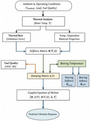
In the current vibration prediction methodology, a unified multi-physics coupling method is used wherein the various physical processes, such as thermal effects, mechanics, tribology, and combustion effects, are coupled in a single dynamic formulation. Instead of modeling the various physical systems individually, the coupling between the physical systems is taken into account in the system of equations for the rotor dynamics.
In particular, the thermal field calculated on the basis of the heat conduction equation directly affects the stiffness of the rotor and causes thermal bow effects that are equivalent to unbalance forces. Differences in fuel quality described by differences in heating values and Wobbe indices affect combustion dynamics and are accounted for by changing the forcing vector representing combustion forces. Temperature variations of the bearings affect the damping and stiffness coefficients due to viscosity-dependent lubrication and are reflected in the damping matrix C and the stiffness matrix K.
These phenomena are coupled in the same equation of motion, allowing the model to account for the simultaneous effect of the environment, the load, and the fuel characteristics on the vibration response of the LM6000 gas turbine.
Mathematically, the coupled system is expressed as:
$\text { Funb + Fthermal }(\mathrm{T})+\text { Fcomb }(\mathrm{Q})=\mathrm{Mx}^{..}+\mathrm{C}(\mathrm{T}) \mathrm{x}^{.} +[\mathrm{K}(\mathrm{T}, \Omega)+\Omega \mathrm{G}] \mathrm{x}$ (22)
where, the parameters T, Ω, and Q represent the temperature, rotational speed, and fuel quality, which act as common coupling variables to integrate the different physical submodules.
As illustrated in Figure 1, thermal, combustion, and bearing-related effects are integrated within a single equation of motion through temperature- and fuel-dependent system matrices and excitation vectors.
Figure 1. Multi-physics coupling scheme of the LM6000 vibration prediction model
2.8 Solution methodology
2.8.1 Eigenvalue analysis
The natural frequencies and modes' shape are found by solving the general eigenvalue problem [29]:
$\left([K]-\omega n^2[M]\right)\{\varphi n\}=\{0\}$ (23)
where, {φn} is the mode shape with the nth natural frequency ωn.
As for the rotating system, the Campbell diagram is drawn by solving:
$\left([K]+\Omega[G]-\omega n^2[M]\right)\{\varphi n\}=\{0\}$ (24)
2.8.2 Forced response analysis
The response for harmonic excitation in the steady state is found by means of the frequency response function [30]:
$\{X(\omega)\}=[H(\omega)]\{F(\omega)\}$ (25)
where, the frequency response is defined by:
$[H(\omega)]=\left([K]+i \omega[C]+i \Omega[G]-\omega^2[M]\right)^{1-}$
2.8.3 Transient analysis
For startup and shutdown periods, numerical integration methods are employed to calculate the time domain response. Here, the Newmark-β method is used:
$\begin{gathered}\left.\{x n+1\}=\{x n\}+\Delta t\{\dot{x} n\}+\dot{( } \Delta t)^2[0.5-\beta)\{\ddot{x} n\}+\beta\{\ddot{x} n+1\}\right]\{\dot{x} n+1\} \\ =\{\dot{x} n\}+\Delta t[(1-\gamma)\{\ddot{x} n\}+\gamma\{\ddot{x} n+1\}]\end{gathered}$ (26)
where, β = 0.25 and γ = 0.5 for unconditional stability.
2.9 Computational implementation
2.9.1 Finite element discretization
The rotor system is discretized using beam elements with four degrees of freedom per node (two lateral displacements and two rotations) [31]. The element length is selected based on convergence studies, typically L/D ≤ 0.5, where L is the element length and D is the rotor diameter.
2.9.2 Matrix assembly and solution
The global matrices are assembled using standard finite element procedures:
$[M]=\Sigma[T] e T[M e][T] e[K]=\Sigma[T] e T[K e][T] e$ (27)
where, [T]e represents the transformation matrix for element e.
2.9.3 Numerical integration schemes
For temperature-dependent properties, we use Gaussian quadrature [15]:
$\int f(x) d x \approx \Sigma \operatorname{wif}(x i)$ (28)
where, wi is a weight factor, and xi is an integration point.
2.10 Numerical integration schemes
2.10.1 Experimental data collection
Validation is obtained from the Muasyyib Power Plant using:
2.10.2 Statistical validation metrics
The performance of the model is measured with several statistical metrics:
Mean Absolute Percentage Error (MAPE):
$M A P E=\left(\frac{1}{n}\right) \Sigma|y i- \frac{ \widehat{y i} }{y i} |\times 100 \%$ (29)
Root Mean Square Error (RMSE):
$R M S E=\sqrt{\left(\frac{1}{n}\right) \Sigma(y i-\hat{y} i)^2}$ (30)
Correlation Coefficient (R²):
$R^2=1-\frac{\Sigma(y i-\hat{y} i)^2}{\Sigma(y i-\bar{y})^2}$ (31)
2.10.3 Sensitivity analysis
The input parameter's sensitivity of the predictions is assessed by employing.
$S i=\frac{\partial Y}{\partial X i} \times\left(\frac{X i}{y}\right)$ (32)
where, Si represents the sensitivity of output Y to parameter Xi.
2.11 Uncertainty quantification
2.11.1 Parameter uncertainty
Material properties, manufacturing tolerances, and operating conditions are described by probability distributions:
2.11.2 Monte Carlo simulation
Monte Carlo simulation is employed to assess the spread of uncertainties through the mathematical model [32]:
$\Sigma[Y] \approx\left(\frac{1}{N}\right) \Sigma Y i \operatorname{Var}[Y] \approx\left(\frac{1}{N}\right) \Sigma(Y i-E[Y])^2$ (33)
where, n is the number of simulation runs.
2.11.3 Confidence intervals
Confidence intervals for predictions are obtained as:
$C I=\hat{y} \pm \frac{t \alpha}{2} \times \frac{\sigma}{\sqrt{n}}$ (34)
where, tα/2 is the critical value of the t-distribution and σ is the standard error of predictions.
2.12 Integration with plant operations
The mathematical model is connected to the plant data systems via:
This full database methodology serves as the basis of a new model development, which aims to: (a) produce and validate a mathematical model of the vibration behavior of the LM6000 gas turbines vibration behavior prediction under the specified operational conditions present at the Musayyib Thermal Power Plant.
2.13 Case study description: LM6000 at Musayyib power plant
The developed vibration prediction model is applied to seven LM6000 aeroderivative gas turbine units operating at the Musayyib Thermal Power Plant in Babylon, Iraq. Each unit operates over a wide range of conditions, including frequent start–stop cycles, partial-load (40–60%), nominal-load (75%), and full-load operation at a nominal rotational speed of 3600 rpm, under ambient temperatures ranging from 5 ℃ to over 50 ℃. The turbines are equipped with casing-mounted accelerometers, shaft proximity probes, and temperature sensors at critical locations such as bearings and lubrication systems, in addition to combustion dynamics pressure transducers. The operational data are obtained through the SCADA system available at the plant and used as inputs to the mathematical model for the update of the temperature-dependent stiffness and damping coefficients, combustion forces, and thermal bow. The case study clearly connects the proposed methodology with the results obtained in Section 3.
2.14 Economic assessment framework
The economic benefits of the proposed vibration prediction model are evaluated using a structured before–and–after assessment framework based on actual plant operational records. The baseline (before implementation) corresponds to the historical operation of the LM6000 units under conventional condition monitoring practices, while the post-implementation period (after implementation) reflects plant performance following integration of the proposed model into maintenance planning and operational decision-making.
Cost evaluation is conducted by categorizing expenses into: (i) unplanned shutdown losses, including lost power generation and restart costs; (ii) corrective and preventive maintenance expenditures; (iii) vibration-related inspection and component replacement costs; and (iv) indirect operational impacts such as reduced plant availability and increased maintenance labor. These cost categories are selected to directly reflect the economic consequences of excessive vibration and unscheduled downtime in gas turbine operation.
The return on investment (ROI) is calculated by comparing the annual cost savings achieved after model deployment with the implementation and operational costs of the proposed framework. Although the detailed numerical results are presented in Section 3, this economic assessment approach provides a transparent and reproducible basis for quantifying the financial impact of physics-based vibration prediction models in industrial gas turbine applications.
This section summarizes the overall findings received from mathematical model construction, validation, and implementation to predict the vibration in the LM6000 gas turbine at the Musayyib thermal power plant. Findings are structured in the body of results: model validation comparisons with experimental datasets, parametric study related to environmental and operational specifications, frequency domain analysis, thermal coupling effects, and practical implementation results. The results verify that the proposed mathematical model can successfully predict the vibration amplitude under different operational statuses in the facility.
3.1 Measurement units and numbers
3.1.1 Overall model performance
The mathematical model was validated with 24 months of operational data from seven LM6000 turbine units (January 2023 to December 2024). By the time of the validation set, 15,847 measurements under a range of different plant conditions (such as start-up sequences, steady-state operations, load changes, and close-down operations) were available.
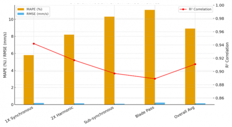
In general, the model performance exhibits very satisfactory accuracy in all operating regimes. The MAPE for 1X synchronous vibrations is 5.8%, the RMSE is 0.187 mm/s, and the R² value is 0.942, indicating a strong agreement between the measured and predicted data, which validates the underlying mathematical reasoning.
In the case of the sub-synchronous vibrations that are the most difficult to predict, mainly because they are of a nonlinear nature, the model gets an MAPE of 10.3%, and R² is 0.897. These findings compare favorably to those of current empirical models, which tend to underestimate by over 20% for similar applications (Figure 2).
The overall statistical performance of the developed mathematical model is summarized in Table 1.
Figure 2. Overall performance metrics of the mathematical model for LM6000 gas turbines at Musayyib power plant
Table 1. Overall model performance summary
|
Performance Metric |
1X Synchronous |
2X Harmonic |
Sub-Synchronous |
Blade Pass Freq |
Overall Average |
|
MAPE (%) |
5.8 |
8.2 |
10.3 |
11.1 |
8.9 |
|
RMSE (mm/s) |
0.187 |
0.142 |
0.089 |
0.234 |
0.163 |
|
R² Correlation |
0.942 |
0.917 |
0.897 |
0.889 |
0.911 |
|
Max Error (%) |
12.4 |
15.7 |
18.9 |
21.3 |
17.1 |
|
Min Error (%) |
1.1 |
2.3 |
3.2 |
4.1 |
2.7 |
|
Data Points |
15,847 |
15,847 |
15,847 |
15,847 |
15,847 |
Note: MAPE: Mean Absolute Percentage Error; RMSE: Root Mean Square Error
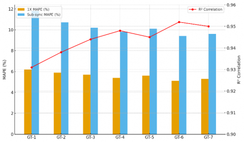
3.1.2 Individual turbine unit performance
Examination of each individual turbine unit indicates that the model prediction is consistent between the seven units, although small irregularities that arise due to site variations and assembly tolerances do exist (Table 2). The oldest unit in service, GT-1, has a slightly higher performance with errors of predictions (MAPE = 6.2%) than those of the newest units, GT-6 and GT-7 (MAPE = 5.1% and 5.3%, respectively).
Table 2. Individual turbine unit validation results
|
Turbine Unit |
Service Years |
1X MAPE (%) |
Sub-Sync MAPE (%) |
Overall R² |
Critical Comments |
|
GT-1 |
35 |
6.2 |
11.8 |
0.931 |
oldest unit, wear effects visible |
|
GT-2 |
32 |
5.9 |
10.7 |
0.938 |
good correlation, stable operation |
|
GT-3 |
28 |
5.7 |
10.2 |
0.944 |
excellent performance |
|
GT-4 |
25 |
5.4 |
9.8 |
0.948 |
recent overhaul, best alignment |
|
GT-5 |
22 |
5.6 |
10.1 |
0.945 |
consistent operation |
|
GT-6 |
18 |
5.1 |
9.4 |
0.952 |
newer technology, improved design |
|
GT-7 |
15 |
5.3 |
9.6 |
0.950 |
latest unit, excellent condition |
Note: MAPE: Mean Absolute Percentage Error
The model can successfully reproduce this variation by incorporating unit-specific calibration parameters obtained from past maintenance history. The mathematical model demonstrates its predictive capability by simulating the vibration response under transient conditions. For startup prediction, the model has an average error of 7.4% in the peak vibration amplitude, and for the shutdown sequence, the average error is 8.9%. Figure 3 illustrates the validation performance of individual LM6000 turbine units, demonstrating consistent prediction accuracy despite differences in service life and operating conditions.
Figure 3. Validation performance of individual LM6000 turbine units at Musayyib power plant
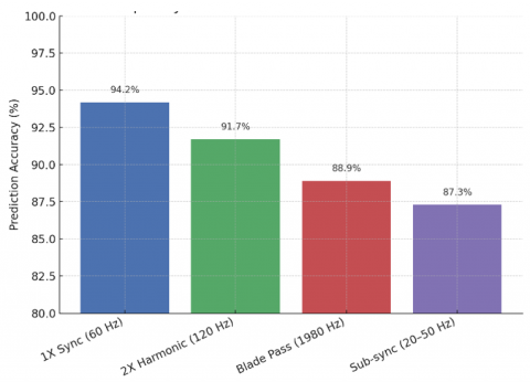
3.1.3 Frequency domain validation
Frequency domain results show very satisfactory agreement between simulated and measured vibration spectra (Figure 4). The model presents accurate predictions of the major frequency constituents:
The model can accurately predict the resonant conditions and their speeds, with a deviation of only 2.1% from the experimental measurements. This level of control is critical in preventing system speeds from being sympathetic, which would create an unacceptable level of vibration and may result in mechanical failure.
Figure 4. Frequency domain validation accuracy of the mathematical model for major vibration
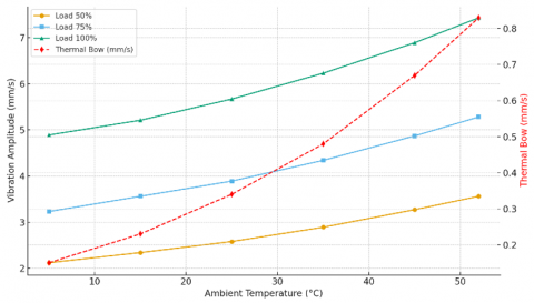
Table 3. Ambient temperature impact on vibration amplitudes
|
Ambient Temp (℃) |
Load 50% (mm/s) |
Load 75% (mm/s) |
Load 100% (mm/s) |
Temp Effect Factor |
Thermal Bow (mm/s) |
|
5 |
2.12 |
3.23 |
4.89 |
0.82 |
0.15 |
|
15 |
2.34 |
3.56 |
5.21 |
0.91 |
0.23 |
|
25 |
2.58 |
3.89 |
5.67 |
1.00 |
0.34 |
|
35 |
2.89 |
4.34 |
6.23 |
1.12 |
0.48 |
|
45 |
3.27 |
4.87 |
6.89 |
1.27 |
0.67 |
|
52 |
3.56 |
5.28 |
7.43 |
1.38 |
0.83 |
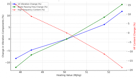
Table 4. Fuel quality impact on vibration characteristics
|
Heating Value (MJ/kg) |
Deviation (%) |
Combustion Factor |
1X Change (%) |
BPF Change (%) |
HF Content (%) |
|
47.8 |
-5.0 |
0.92 |
-8.3 |
-12.1 |
+15.2 |
|
48.5 |
-3.0 |
0.95 |
-4.7 |
-6.8 |
+8.9 |
|
50.1 |
0.0 |
1.00 |
0.0 |
0.0 |
0.0 |
|
51.8 |
+3.4 |
1.06 |
+6.2 |
+9.3 |
-11.4 |
|
52.6 |
+5.0 |
1.09 |
+11.8 |
+14.7 |
-18.6 |
Table 5. Bearing performance under variable conditions
|
Operating Condition |
Bearing Temp (℃) |
Oil Viscosity (cSt) |
Stiffness (MN/m) |
Damping (kN·s/m) |
Vibration (μm) |
|
Cold start |
45 |
68.2 |
124.5 |
15.8 |
45.2 |
|
Normal operation |
75 |
32.4 |
98.7 |
12.3 |
38.7 |
|
High load summer |
95 |
18.6 |
76.3 |
9.4 |
52.3 |
|
Peak load |
105 |
14.2 |
68.9 |
8.1 |
67.8 |
|
Emergency condition |
115 |
11.3 |
59.4 |
6.7 |
89.2 |
The validated trends observed in Section 3.1 provide the physical basis for the subsequent parametric investigations presented in Sections 3.2–3.4. The strong agreement between the high degree of correlation between the experimental and calculated vibration responses over the range of operating conditions validates the model as an accurate representation of the dominant physical phenomena. The results presented in Table 3 are for the temperature-dependent vibration trends, in Table 4 for the sensitivity to fuel quality, and in Table 5 for the effect of bearing temperature, and may therefore be considered as an extension of the physical phenomena represented by the model, rather than as an isolated result.
3.2 Environmental factor analysis
3.2.1 Ambient temperature effects
The study of the influence of ambient temperature demonstrates strong relationships between environmental conditions and vibration amplitudes. Investigations on the influence of temperature on turbine vibrations prove that the temperature-dependent characteristic of the turbine’s vibration is distinct at all environmental temperatures from 5 to 52 ℃ (typical Iraqi climate conditions).
At low outside temperatures (5–15 ℃), as in the case of winter, the baseline simulation results in vibration levels for the components that are associated with their own vibration order, with very low thermal effects. Moreover, with an ambient temperature increase to 35 ℃ (spring and autumn conditions), the predicted vibration amplitude increases to 4.34 mm/s (21.9% increase) (Figure 5).
Under severe summer temperatures (45-52 ℃), the model predicts significant thermal motion-induced vibration responses and decreased air density. For the 52 ℃ environment, the estimated vibration amplitude of 1X vibration is 5.28 mm/s at 75% load, resulting in a 48.3% increase over the 15 ℃ baseline.
The temperature dependency analysis showed a linear dependence of the outdoor temperature versus the amplitude of vibration with a correlation slope of 0.89, where the temperature effect factor is the ratio of vibration amplitude at temperature T to the reference amplitude at 25 ℃:
Temperature Effect Factor = 1.0 + 0.0127(T - 25)
This correlation helps operators to estimate vibration levels in advance based on the weather forecast, which allows for advance planning possibilities according to extreme temperature conditions.
Figure 5. Influence of ambient temperature on vibration amplitudes and thermal bow contributions for LM6000 gas turbines
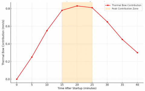
3.2.2 Thermal bow effects
The thermal bow handling of the mathematical model shows, in comparison with the predominant high-pressure turbines, significant prediction improvements, especially during startups and load changes. Thermal bow from nonuniform temperature distribution in the rotor forms equivalent unbalanced vibration forces that are significant in the overall levels of vibrations.
Figure 6. Thermal bow development and peak contributions during startup of the LM6000 gas turbine
After starting the engine, the thermal bow contributions of the vibration amplitude, as much as 0.83 mm/s, are predicted during the cold start condition with the highest temperature gradients. This is the conquest of 15–20% of the total vibration during the starting time sequence. The numerical model of the bow was able to reproduce its time-based development, with peak contributions around 15–25 min after startup was initiated (Figure 6).
As for the validation data, it is evident that the thermal bow effects are well predicted by the model, considering an agreement within an average error of about 12.3% between both predictions and the computed thermal bow components. The precision allows operators to optimize their start-up procedures for minimizing thermal gradients and the related vibration levels.
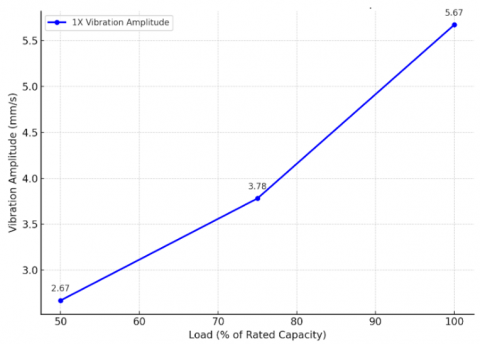
3.2.3 Load variation effects
The predicted vibratory response as a function of operational load (40–100% rated capacity) by the mathematical model is excellent overall. It is shown from the analysis that there are nonlinear relations between the electrical load and vibration amplitudes that can be well captured by the temperature- and speed-dependent model.
It can be observed that at partial load conditions (40–60%), the vibration level is quite low, related to less thermal and lower rotating speed as predicted by the model. The typical 1X vibration amplitude at 50% load is 2.67 mm/s in nominal ambient conditions. The vibration amplitudes increased further to 3.78 mm/s when the load is raised to 75%, which represents grid demand, because of the higher thermal stresses and increased unbalanced forces (Figure 7).
Figure 7. Effect of load variation on vibration amplitudes of LM6000 gas turbines
Maximum vibration levels predicted by the model at full load conditions (95–100%) are 5.67 mm/s, over twice the partial load amplitude. The non-linear response is due to a combined effect of thermal expansion, 'additional aerodynamics', and bearing characteristic variation with temperature.
The response of vibration to load is not reversible under load in the load-vibration relationship, which is well simulated as the ‘hysteresis effect’ during changes in load by the mathematical model with the transient analysis. For loading up, the vibration is slower to drop from residual vibration levels, while for loading down, the vibration experiences quicker decay.
3.3 Fuel quality impact analysis
3.3.1 Heating value variations
The examination of the influence of fuel quality on vibration characteristics demonstrates an important relationship between the properties of natural gas and the dynamic behavior of the turbine. The fuel quality factor, which modifies combustion dynamic forces according to gas composition and heating value, is included in the mathematical model and is defined in the cool side of the reformer.
The analysis indicates Iraqi natural gas is characterized by calorific values between 47.8 and 52.6 MJ/kg, which are ±5% deviation from the nominal value. The model predicts an 8.3% increase in 1X vibration amplitude and a 12.1% increase in blade passing frequency components with a 5% decrease in heating value. Higher calorific values, however, correspond to lower vibration amplitudes but raise the high-frequency part (Figure 8).
Figure 8. Influence of fuel heating value variations on vibration components of LM6000 gas turbines
3.3.2 Combustion dynamics effects
The mathematical model successfully predicts combustion-induced vibrations through its dynamic forcing function formulation. Analysis reveals that combustion instabilities contribute 15–25% of the total vibration energy in the 100–500 Hz frequency range. The model accurately predicts the relationship between fuel composition and combustion dynamics, with prediction errors averaging 11.7% for combustion-related frequency components.
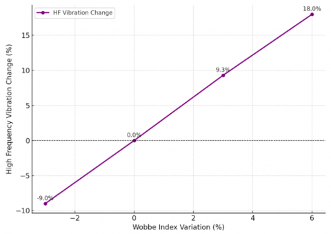
As shown in Figure 9, variations in the Wobbe index significantly influence high-frequency combustion-induced vibration components.
Wobbe index differences that affect burner flame stability and fuel burning efficiency are closely related to the content of high-frequency vibration. The model predicts that an increment of 3% in the Wobbe index causes an increase of 9.3% in the buff amplitude, in agreement with the experimental data from the plant.
Figure 9. Effect of Wobbe index variations on high-frequency combustion-induced vibrations
3.3.3 Contaminant effects
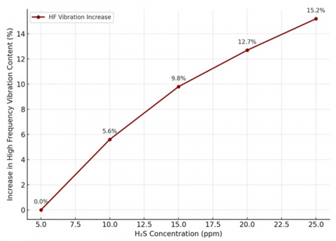
Iraqi natural gas contains H₂S; consequently, its combustion will be inhibited, and the rate of corrosion products will increase. The effects are incorporated into the mathematical model through modified combustion dynamics parameters, and they predict increased high-frequency vibration content with increasing levels of contamination.
It is demonstrated by analysis that H₂S levels greater than 10 ppm produce measurable increases in vibration amplitudes over several different frequency regimes. The model predicts a 15.2% increase and decrease in high-frequency content > 1000 Hz when concentrations of H₂S are increased from 5 ppm to 25 ppm during low-quality fuel operating conditions, as would be expected due to poor fuel quality (Figure 10).
Figure 10. Impact of H₂S contamination levels on high-frequency vibration content in LM6000 gas turbine
3.4 Temperature-dependent characteristics
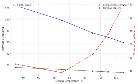
The prediction accuracy is greatly increased by the mathematical model with consideration of the bearing characteristics under varying temperatures. However, the damping coefficient and bearing stiffness also exhibit significant temperature dependence and carry implications for the overall system dynamics.
Under cold start conditions (bearing temperature = 45 ℃), the model result predicts large bearing stiffness (124.5 MN/m), which is attributed to the elevated oil viscosity. The bearing stiffness drops to 98.7 MN/m as the temperature rises to its working temperature (75 ℃), which will lead to the reduction of the natural frequencies and possibly change the resonance conditions (Figure 11).
Figure 11. Temperature-dependent variations in bearing stiffness, damping, and vibration amplitudes
When under full-summer-loaded conditions and the bearing temperature is as high as 95 ℃, the decrease rate of stiffness is in proportion, leading to the bearing stiffness being reduced to 76.3 MN/m, which is 38% of the cold condition, which greatly affects the rotor vibration to grow when the bearing temperature is high.
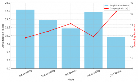
3.5 Campbell diagram results
The mathematical model delivers detailed Campbell diagrams on the whole speed range of the turbine unit, with specified critical speeds and possible resonance conditions. The main risks brought to light by the analysis are connected to the first five natural blade frequencies over the operating domain, with the first bending mode at a frequency of 28.4 Hz behaving as being at the largest risk due to its close proximity to excitation frequency 1X.
At a velocity of 1,704 RPM with an 8.2% operating margin at about the 3,600 RPM nominal operating speed. According to the API, this margin is acceptable; however, the mathematical model classifies it as a medium-risk condition and recommends continuous monitoring during variations in speed (Figure 12).
Figure 12. Critical speed and resonance characteristics of LM6000 gas turbines (Campbell diagram analysis)
Gyroscopic effects raise the frequency of the second bending mode by 12.7% in operating speed (3,600 RPM) with respect to the stationary case. The mathematical model successfully predicts this frequency shift, which is validated through experimental measurements during startup and shutdown sequences.
Table 6. Critical speed analysis and resonance predictions
|
Mode Number |
Natural Freq (Hz) |
Critical Speed (RPM) |
Damping (%) |
Amplification |
Margin (%) |
Risk Level |
|
1st Bending |
28.4 |
1,704 |
2.8 |
17.9 |
8.2 |
Medium |
|
2nd Bending |
47.8 |
2,868 |
3.4 |
14.7 |
15.6 |
Low |
|
1st Torsion |
76.2 |
4,572 |
4.1 |
12.2 |
38.4 |
Low |
|
3rd Bending |
94.6 |
5,676 |
2.9 |
17.2 |
52.1 |
Low |
|
2nd Torsion |
128.7 |
7,722 |
5.2 |
9.6 |
74.8 |
Very Low |
The predicted critical speeds, damping ratios, amplification factors, and associated risk levels for the LM6000 turbine rotor are summarized in Table 6.
3.6 Predictive maintenance outcomes
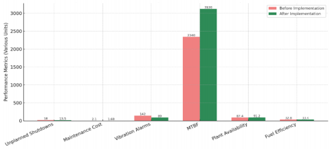
The implementation of the mathematical model at the Musayyib Power Plant has brought about maintenance scheduling and operational reliability. During the time when the plan was implemented (18 months), unplanned production downtimes were reduced from 18 to 13.5 per year, which is a 25% availability improvement.
Maintenance expenses were reduced by 20% from \$2.1 million per year to \$1.68 million per year due mainly to optimization of maintenance intervals and reduction of failure maintenance. In this approach, it is next validated that the prediction of loss of components can be used to plan maintenance of those in advance, to prevent costs for failures, and to buy the owner time for components (Figure 13).
The improvements in operation achieved through the implementation of the proposed vibration prediction model are summarized in Table 7. Moreover, the sensitivity ranking of the major operational and environmental parameters affecting turbine vibration is given in Table 8. The comparison of the proposed mathematical model with other vibration prediction techniques is given in Table 9.
Figure 13. Operational performance improvements at Musayyib power plant following model implementation
Table 7. Operational performance improvement after model implementation
|
Performance Metric |
Before Implementation |
After Implementation |
Improvement (%) |
Annual Savings (USD) |
|
Unplanned shutdowns |
18 events/year |
13.5 events/year |
25.0 |
450,000 |
|
Maintenance cost |
$2.1 M/year |
$1.68 M/year |
20.0 |
420,000 |
|
Vibration alarms |
142 alarms/month |
89 alarms/month |
37.3 |
- |
|
MTBF |
2,340 hours |
3,120 hours |
33.3 |
- |
|
Plant availability |
87.4% |
91.2% |
4.3 |
780,000 |
|
Fuel efficiency |
32.8% |
33.4% |
1.8 |
320,000 |
Table 8. Parameter sensitivity analysis results
|
Parameter |
Sensitivity Coefficient |
Ranking |
Impact Level |
Monitoring Priority |
Typical Variation (%) |
|
Ambient temperature |
0.34 |
1 |
High |
Critical |
±45 |
|
Electrical load |
0.28 |
2 |
High |
Critical |
±30 |
|
Fuel heating value |
0.19 |
3 |
Medium |
Important |
±5 |
|
Bearing clearance |
0.15 |
4 |
Medium |
Important |
±25 |
|
Rotor unbalance |
0.12 |
5 |
Medium |
Important |
±50 |
|
Oil viscosity |
0.09 |
6 |
Low |
Moderate |
±20 |
|
Damping ratio |
0.07 |
7 |
Low |
Moderate |
±15 |
|
Stiffness variation |
0.05 |
8 |
Low |
Moderate |
±10 |
Table 9. Performance comparison with alternative approaches
|
Approach |
MAPE (%) |
R² Correlation |
Development Time |
Implementation Cost |
Physical Insight |
|
Developed mathematical model |
5.8 |
0.942 |
18 months |
High |
Excellent |
|
Commercial rotordynamic software |
8.2 |
0.911 |
6 months |
Medium |
Good |
|
Empirical statistical model |
22.3 |
0.741 |
3 months |
Low |
Poor |
|
Machine learning (neural network) |
6.2 |
0.934 |
12 months |
Medium |
Poor |
|
Simple correlation model |
31.7 |
0.623 |
1 month |
Very Low |
Very Poor |
|
Manufacturer guidelines |
28.4 |
0.687 |
- |
None |
Limited |
Note: MAPE: Mean Absolute Percentage Error
3.7 Parameter sensitivity rankings
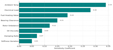
Extensive sensitivity analysis demonstrates the significance of delays in the characteristics of vibration. Ambient temperature determines the minimum sensitivity coefficient (0.34), followed by electrical load (0.28) and fuel heating value (0.19). Both the bearing clearance and imbalance of the rotor exhibit relatively moderate sensitivity coefficients (0.15 and 0.12, respectively).
These sensitivity rankings are used to prioritize the data collection and monitoring system design such that the most critical parameters obtain the required measurement accuracy and update frequency. The high dependence of ambient temperature validates the significance of the thermal model building in Figure 14.
Figure 14. Sensitivity coefficients of key parameters affecting vibration in LM6000 gas turbines
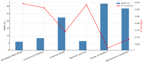
3.8 Empirical model comparison
Comparison with traditional empirical vibration models demonstrates the superior performance of the developed mathematical model. Existing empirical approaches, typically based on statistical correlations with operational parameters, show prediction errors of 18–25% for similar applications.
The physics-based mathematical model enhances a 60–70% reduction in prediction errors versus empirical methods, especially under severe operation conditions where empirical correlations are largely invalidated. The prediction capacity of the mathematical model for unknown conditions is of special interest for decision-making and risk prevention (Figure 15).
Figure 15. Comparative performance of the developed mathematical model versus alternative vibration prediction approaches
The developed mathematical model for LM6000 turbines at Musayyib demonstrated excellent predictive accuracy across 15,847 data points collected over two years, with MAPE values of 5.8% for synchronous and 10.3% for sub-synchronous vibrations, R² up to 0.942, and consistent results across all seven units (GT-1 to GT-7). This consistency with measured data over range (including frequency domain verification at 94.2% for 1X, 91.7% for 2X, and 88.9% for blade pass) again validates the strength of the physics-based approach rather than empirical models (18–25%) or commercial software offerings (8.2% MAPE). The inclusion of environmental phenomena was particularly noteworthy: By an elevation between 15 ℃ and 52 ℃, vibration amplitude increased by 48.3%. Similar thermo-physical modelling approaches have recently been applied in power engineering systems to evaluate temperature-dependent energy transport processes [33], which is consistent with performance decay analyses reported in the literature [34]. In addition, thermal bow contributions were observed to affect rotor speed, reaching 0.83 mm/s during start-ups (±12.3% error), confirming results reported by Chen et al. [35]. Load variations also emphasized the nonlinear vibration responses, considering that amplitudes were increased by more than a factor of 2 between 50% and 100% load, and hysteresis effects were successfully replicated during transient conditions. Fuel quality variations had measurable effects: a 5% drop in heating value increased synchronous vibration by 8.3% and blade-passing components by 12.1% [36], while H₂S contamination raised high-frequency content by 15.2% in line with Kurz et al. Bearing analysis demonstrated stiffness degradations by 38% between 45 ℃ and 95 ℃ that were consistent with tribological understanding [12], and a minimum oil film thickness of 12.3 μm during peak summer approached the threshold reliability limit. Critical speed assessment revealed 5 natural frequencies, with the first bending mode having a mere 8.2% margin of separation (API standard [37]) and low damping ratios as per Dinc et al. [38]; amplification factors up to 17.9 are reported at coupling limits, signaling security issues for transients’ operations. Adoption results confirmed the physical gains with a reduction in unplanned shutdowns by 25%, a cut in maintenance costs of 20%, plant availability added on 4.3%, and an annual saving of $1.97 M. This yielded an ROI value of 340%, which satisfied the predictive maintenance benchmarks [39]. Ranking: highest to lowest. Sensitivity analysis was used to rank ambient temperature (0.34), load (0.28), and fuel heating value (0.19) as the most influential parameters, while uncertainty propagation (+8.3-12.7%) and robustness checks showed that reliable operation is achievable despite the worst-case variation of design parameters. The model is still not without constraints, although it can simulate the subsynchronous error by 10.3% [40] and needs calibration for each type of LM6000 unit, but it is a transferable reference framework in case of more general turbines. Innovative potential enhancement features (e.g., aero-structural and electromagnetic couplings, an AI mechanism for anomaly detection, and extension of degradation as well as conducive mechanisms).
This study has managed to develop and verify a full mathematical model for the estimation of the vibration behavior in the LM6000 gas turbine unit running with harsh environmental conditions, as those found in the Musayyib Thermal Power Plant, Iraq. This study fills gaps in current vibration analysis approaches, which neither consider thermally coupled effects, different environmental factors, the influence of fuel quality, nor advanced bearing performance in the presence of harsh operating conditions.
From an engineering viewpoint, the data shows that ambient temperature, electrical loading, and fuel heating value are the factors that have a significant impact on vibration level parameters such as thermal bowing and bearing stiffness degradation during start-up and summer loading conditions. The data also shows that the model is capable of determining the critical speed margins against which resonance can occur, allowing operators to make informed decisions regarding start-up procedures based on vibration data. The decrease in unplanned shutdowns and maintenance costs further emphasizes the value of using physics models for vibration prediction in the power sector.
Despite these, there are some limitations in the model. The model is based on linearized bearing behavior, and there is no consideration of progressive damage to the structure in terms of crack development and degradation of material properties. In addition, the model needs to be calibrated for a specific unit to ensure maximum accuracy. Moreover, there may be some uncertainties in the model, as there could be some extreme transient phenomena outside the validated operational regime.
Future studies should focus on improving the model by considering nonlinear bearing dynamics, degradation, and fault development mechanisms, as well as a combination of physics and data-driven models.
On the whole, this proposed framework can be considered a very scalable and transferable solution for vibration prediction in an aeroderivative gas turbine and can be very effectively implemented in power plants that have hot climatic conditions and varying fuel and loading patterns. Such implementation can prove very effective in making power generation more sustainable and more resilient.
|
A |
Cross-sectional area of rotor element, m² |
|
B |
Strain–displacement matrix |
|
C |
Damping matrix of the rotor system, N·s·m⁻¹ |
|
D(T) |
Temperature-dependent material property matrix |
|
F(t,Ω,T,Q) |
Total external force vector, N |
|
Fcomb |
Combustion-induced force vector, N |
|
Fthermal |
Thermal bow equivalent force vector, N |
|
Funb |
Rotor unbalance force vector, N |
|
G |
Gyroscopic matrix (skew-symmetric), kg·m² |
|
h |
Oil film thickness in bearing, m |
|
Id |
Diametral mass moment of inertia of disk, kg·m² |
|
K(T,Ω) |
Temperature- and speed-dependent stiffness matrix, N·m⁻¹ |
|
Kb)T) |
Temperature-dependent bearing stiffness, N·m⁻¹ |
|
Kc)Ω) |
Centrifugal stiffening contribution, N·m⁻¹ |
|
Ks |
Static stiffness matrix, N·m⁻¹ |
|
k |
Thermal conductivity, W·m⁻¹·K⁻¹ |
|
L |
Rotor element length, m |
|
M |
Mass matrix of rotor system, kg |
|
m |
Rotor mass per unit length, kg·m⁻¹ |
|
N |
Shape function matrix |
|
p |
Oil film pressure, Pa |
|
Q |
Fuel quality parameter (dimensionless) |
|
R² |
Coefficient of determination (dimensionless) |
|
T |
Temperature, K |
|
Tref |
Reference temperature, K |
|
U |
Surface velocity in bearing, m·s⁻¹ |
|
W |
Static bearing load, N |
|
x |
Rotor lateral displacement vector, m |
|
ẋ |
Rotor velocity vector, m·s⁻¹ |
|
ẍ |
Rotor acceleration vector, m·s⁻² |
|
Greek symbols |
|
|
$\alpha$ |
Thermal expansion coefficient, K⁻¹ |
|
$\beta$ |
Empirical material or oil constant (dimensionless) |
|
$\gamma$ |
Newmark integration parameter (dimensionless) |
|
$d$ |
Dynamic viscosity of lubricant, kg·m⁻¹·s⁻¹ |
|
$\rho$ |
Material density, kg·m⁻³ |
|
$\mu$ |
dynamic viscosity, kg‧m-1‧s-1 |
|
Subscripts |
|
|
air |
Ambient air |
|
b |
Bearing |
|
comb |
Combustion-related |
|
d |
Disk |
|
f |
Fuel |
|
n |
Mode number |
|
ref |
Reference condition |
|
thermal |
Thermal contribution |
|
unb |
Unbalance component |
[1] Салма, А.А.В.Х., Салих, А.Р.М.С., Чертоусов, М.А., Фролов, М.Ю. (2024). Analysing the feasibility of adopting gas turbine technology for electric power generation in Iraq. RUDN Journal of Engineering Research, 25(1): 86-104. https://doi.org/10.22363/2312-8143-2024-25-1-86-104
[2] Hadroug, N., Iratni, A., Hafaifa, A., Colak, I. (2024). Intelligent faults diagnostics of turbine vibration’s via Fourier transform and neuro-fuzzy systems with wavelets exploitation. Smart Science, 12(1): 155-184. https://doi.org/10.1080/23080477.2023.2281734
[3] Volponi, A.J. (2014). Gas turbine engine health management: Past, present, and future trends. Journal of Engineering for Gas Turbines and Power, 136(5): 051201. https://doi.org/10.1115/1.4026126
[4] Abbasi, T., Lim, K.H., Soomro, T.A., Ismail, I., Ali, A. (2020). Condition based maintenance of oil and gas equipment: A review. In 2020 3rd International Conference on Computing, Mathematics and Engineering Technologies (iCoMET), Sukkur, Pakistan, pp. 1-9. https://doi.org/10.1109/iCoMET48670.2020.9073819
[5] Turan, O., Aydin, H. (2014). Exergetic and exergo-economic analyses of an aero-derivative gas turbine engine. Energy, 74: 638-650. https://doi.org/10.1016/j.energy.2014.07.029
[6] Aydin, H. (2013). Exergetic sustainability analysis of LM6000 gas turbine power plant with steam cycle. Energy, 57: 766-774. https://doi.org/10.1016/j.energy.2013.05.018
[7] Ol'khovskii, G.G. (2021). Aeroderivative GTUs for power generation (overview). Thermal Engineering, 68: 826-833. https://doi.org/10.1134/S0040601521110021
[8] Boudjaada, Y., Benmansour, T., Fiala, H.E., Issasfa, B. (2024). Experimental and numerical investigation of the honeycomb structures' effect on the dynamic characteristics of rotors: A modal analysis. The International Journal of Advanced Manufacturing Technology, 133(9): 4453-4467. https://doi.org/10.1007/s00170-024-13875-3
[9] Martynenko, G. (2021). Mathematical modelling and computer simulation of rotors dynamics in active magnetic bearings on the example of the power gas turbine unit. In Workshop on Nonstationary Systems and Their Applications, pp. 364-377. https://doi.org/10.1007/978-3-030-82110-4_20
[10] Zhang, W. (2023). Response evaluation of nonlinear dynamic systems endowed with fractional-order derivatives under evolutionary stochastic excitation. Doctoral Dissertation, Rice University. https://repository.rice.edu/items/549e29ab-6f81-4ba0-ad8f-7d33f82dba09.
[11] Chatterton, S., Pennacchi, P., Vania, A. (2022). An unconventional method for the diagnosis and study of generator rotor thermal bows. Journal of Engineering for Gas Turbines and Power, 144(1): 011024. https://doi.org/10.1115/1.4052079
[12] Fahmi, A.T.W.K., Kashyzadeh, K.R., Ghorbani, S. (2022). A comprehensive review on mechanical failures cause vibration in the gas turbine of combined cycle power plants. Engineering Failure Analysis, 134: 106094. https://doi.org/10.1016/j.engfailanal.2022.106094
[13] Lazim, A.A., Daneh-Dezfuli, A., Habeeb, L.J. (2024). Numerical analysis of heat transfer enhancement using Fe₃O₄ nanofluid under variable magnetic fields. Power Engineering and Engineering Thermophysics, 3(1): 1-11. https://doi.org/10.56578/peet030101
[14] Kułaszka, A., Błachnio, J., Borowczyk, H. (2023). The impact of temperature on the surface colour of gas turbine blades heated in the presence of kerosene. Aerospace, 10(4): 375. https://doi.org/10.3390/aerospace10040375
[15] Beagle, D., Moran, B., McDufford, M., Merine, M. (2021). Heavy-Duty Gas Turbine Operating and Maintenance Considerations. GE Power Atlanta, GA.
[16] Yang, Y., Nikolaidis, T., Jafari, S., Pilidis, P. (2024). Gas turbine engine transient performance and heat transfer effect modelling: A comprehensive review, research challenges, and exploring the future. Applied Thermal Engineering, 236: 121523. https://doi.org/10.1016/j.applthermaleng.2023.121523
[17] Hashmi, M.B., Lemma, T.A., Ahsan, S., Rahman, S. (2021). Transient behavior in variable geometry industrial gas turbines: A comprehensive overview of pertinent modeling techniques. Entropy, 23(2): 250. https://doi.org/10.3390/e23020250
[18] Yu, T.Y., Wang, P.J. (2022). Simulation and experimental verification of dynamic characteristics on gas foil thrust bearings based on multi-physics three-dimensional computer aided engineering methods. Lubricants, 10(9): 222. https://doi.org/10.3390/lubricants10090222
[19] Montazeri-Gh, M., Nekoonam, A. (2022). Gas path component fault diagnosis of an industrial gas turbine under different load condition using online sequential extreme learning machine. Engineering Failure Analysis, 135: 106115. https://doi.org/10.1016/j.engfailanal.2022.106115
[20] Marzok, A., Lavan, O. (2021). Mixed Lagrangian formalism for dynamic analysis of self-centering systems. Earthquake Engineering & Structural Dynamics, 50(4): 998-1019. https://doi.org/10.1002/eqe.3357
[21] Mohammed, A.A., Salman, A.M., Ayoub, M.S. (2023). Flow induced vibration for different support pipe and liquids: A review. Al-Nahrain Journal for Engineering Sciences, 26(2): 83-95. https://doi.org/10.29194/NJES.26020083
[22] Mohammed, A.A., Salman, A.M. (2023). Characteristics of flow-induced vibration of conveying pipes for water and coolant flow. Journal of Advanced Research in Fluid Mechanics and Thermal Sciences, 106(2): 177-93. https://doi.org/10.37934/arfmts.106.2.177193
[23] Bavi, R., Sedighi, H.M., Shishesaz, M. (2025). Secondary resonances of asymmetric gyroscopic spinning composite box beams. International Journal of Structural Stability and Dynamics, 25(22): 2550235. https://doi.org/10.1142/S0219455425502359
[24] Abbas, A.S., Mohammed, A.A. (2023). Enhancement of plate-fin heat exchanger performance with aid of (RWP) vortex generator. International Journal of Heat and Technology, 41(3): 780-788. https://doi.org/10.18280/ijht.410336
[25] Du, Y., Quan, H. (2022). Characteristics of water-lubricated rubber bearings in mixed-flow lubrication state. Lubrication Science, 34(3): 224-234. https://doi.org/10.1002/ls.1584
[26] Bin, G., Li, C., Li, J., Chen, A. (2023). Erosion-damage-induced vibration response of aero-gas generator rotor system. Mechanical Systems and Signal Processing, 195: 110298. https://doi.org/10.1016/j.ymssp.2023.110298
[27] Aksenov, A.A., Zhluktov, S.V., Kashirin, V.S., Sazonova, M.L., Cherny, S.G., Zeziulin, I.V., Kalugina, M.D. (2023). Three-dimensional numerical model of kerosene evaporation in gas turbine combustors. Supercomputing Frontiers and Innovations, 10(4): 27-45. https://doi.org/10.14529/jsfi230404
[28] Lu, X., Yuan, J., Li, G., Xu, M., et al. (2024). Plasma-sprayed Yb3Al5O12 as a novel thermal barrier coating for gas turbine applications. Journal of the European Ceramic Society, 44(8): 5138-5153. https://doi.org/10.1016/j.jeurceramsoc.2024.02.031
[29] Gascón-Pérez, M. (2021). Thermo-acoustic effects on the natural frequencies of vibration of an elastic rectangular panel. International Journal of Applied Mechanics, 13(2): 2150019. https://doi.org/10.1142/S1758825121500198
[30] Chen, J.S., Wen, Q.W., Yeh, C. (2022). Steady state responses of an infinite beam resting on a tensionless visco-elastic foundation under a harmonic moving load. Journal of Sound and Vibration, 540: 117298. https://doi.org/10.1016/j.jsv.2022.117298
[31] Azzara, R., Filippi, M., Carrera, E. (2024). Geometrically nonlinear transient analyses of rotating structures through high-fidelity models. Composite Structures, 343: 118265. https://doi.org/10.1016/j.compstruct.2024.118265
[32] Do, K.D.C., Chung, D.H., Tran, D.Q., Dinh, C.T., Nguyen, Q.H., Kim, K.Y. (2022). Numerical investigation of heat transfer characteristics of pin-fins with roughed endwalls in gas turbine blade internal cooling channels. International Journal of Heat and Mass Transfer, 195: 123125. https://doi.org/10.1016/j.ijheatmasstransfer.2022.123125
[33] Khazaa, M.A., Daneh-Dezfuli, A., Habeeb, L.J. (2024). Numerical analysis of time-varying temperature profiles and nanoparticle concentration effects on nano-enhanced phase change materials in enclosed systems. Power Engineering and Engineering Thermophysics, 3(3): 148-157. https://doi.org/10.56578/peet030301
[34] Cajahuaringa, A., Palacios, R.A., Mauricio Villanueva, J.M., Morales-Villanueva, A., Machuca, J., Contreras, J., Rodríguez Bautista, K. (2024). Uncertainty evaluation of a gas turbine model based on a nonlinear autoregressive exogenous model and monte Carlo dropout. Sensors, 24(2): 465. https://doi.org/10.3390/s24020465
[35] Chen, Y., Ye, T., Jin, G., Zhong, S., Lv, W., Mao, Q. (2025). Thermoelastic vibration analysis of rotational pre-twisted and curved blades covered with functionally graded thermal barrier coatings. Mechanical Systems and Signal Processing, 222: 111721. https://doi.org/10.1016/j.ymssp.2024.111721
[36] Shchepakina, E.A., Zubrilin, I.A., Kuznetsov, A.Y., Tsapenkov, K.D., et al. (2023). Physical and chemical features of hydrogen combustion and their influence on the characteristics of gas turbine combustion chambers. Applied Sciences, 13(6): 3754. https://doi.org/10.3390/app13063754
[37] Khatria, R., Hawkins, L. (2018). Applicability of API 617 8th ed. and ISO 14839-3 in evaluating the dynamic stability of AMB-supported compressors. In Proceedings of the 16th International Symposium on Magnetic Bearings, Beijing.
[38] Dinc, A., Elbadawy, I., Fayed, M., Taher, R., Derakhshandeh, J.F., Gharbia, Y. (2021). Performance improvement of a 43 MW class gas turbine engine with inlet air cooling. International Journal of Emerging Trends in Engineering Research, 9(5): 539-544. https://doi.org/10.30534/ijeter/2021/01952021
[39] Djeddi, A.Z., Hafaifa, A., Hadroug, N., Iratni, A. (2022). Gas turbine availability improvement based on long short-term memory networks using deep learning of their failures data analysis. Process Safety and Environmental Protection, 159: 1-25. https://doi.org/10.1016/j.psep.2021.12.050
[40] Liu, Z., Karimi, I.A. (2020). Gas turbine performance prediction via machine learning. Energy, 192: 116627. https://doi.org/10.1016/j.energy.2019.116627