Karthik Machahalli Shivarudraiah![]() | Mangalpady Aruna
| Mangalpady Aruna![]() | Ramachandran Thulasiram
| Ramachandran Thulasiram![]() | Swetarani Biswal
| Swetarani Biswal![]() | Polaepalli Siva Kota Reddy*
| Polaepalli Siva Kota Reddy*![]()
© 2026 The authors. This article is published by IIETA and is licensed under the CC BY 4.0 license (http://creativecommons.org/licenses/by/4.0/).
OPEN ACCESS
The present study introduces and validates a novel instrument for measuring the thermal conductivities of electrically conductive and nonconductive liquids under transient conditions. A U-shaped platinum-rhodium wire was employed in the innovative device to function as both a heating element and a temperature sensor, facilitating rapid and accurate measurements. The temperature fluctuation measurement and heating impulse were regulated using a custom-designed electronic circuit and data acquisition system. To validate the apparatus, the thermal conductivities of various liquids were measured: water, alkaline water (pH = 13), and acidic water (pH = 1), representing electrically conductive liquids, and SAE-5W-30 engine oil and transformer oil, representing electrically non-conductive liquids. The measured results were in close agreement with the established reference values. The thermal conductivities of water, SAE-5W-30 engine oil, alkaline water (pH = 13), acidic water (pH = 1), and transformer oil were 0.58, 0.313, 0.59, 0.63, and 0.148 W/m·K, respectively. The standard uncertainty of the developed device was ±2.4%. Each measurement was completed within one second. The proposed method presents several significant advantages over existing techniques, including operational simplicity and cost-effectiveness, as an alternative to current methods. The U-shaped sensor enhances the sensitivity, spatial resolution, and adaptability across diverse applications. Additionally, contemporary electronic instrumentation provides improved precision and accuracy while reducing sample exposure times.
thermal conductivity, sensor unit, electronic component, transient technique, electrically conductive and non-conductive liquids
The thermal conductivity of liquids is a complex property, showing great variability between electrically conductive and non-conductive (insulating) liquids due to differences in how heat is conducted through each type of liquid. These differences have created opportunities for many kinds of applications to use these properties in energy storage, refrigeration, and chemical processing. The reason for the increased thermal conductivities of electrically conductive (ionic and/or liquid metals) liquids is that the charged particles that create the free flow of electrons in these liquids can provide greater efficiency for heat transport than the molecular vibrational mechanisms that transfer heat by conduction in non-conductive (insulating) liquids (such as oils and organic solvents). The thermal characteristics of both kinds of liquid are important to understand if you are trying to create or optimize systems that require precise temperature control, for example, for electronic cooling or heat exchangers [1, 2].
Various industries have studied the thermal conductivity of electrically conductive water. Conductors, such as ions, salts, and nanoparticles, may be added to increase the thermal conductivity of water. Sundar et al. [3] researched the thermal conductivity of Fe3O4 nanoparticles in nanofluids made from water. Their research showed that adding nanoparticles to the fluid greatly increases its thermal conductivity. Therefore, the use of conductive water-based fluids has the potential to be used in heat transfer and cooling applications. In contrast, nonconductive liquids, such as oils, have lower thermal conductivities than conductive liquids. The thermal conductivity of oils at room temperature is between 0.1 W/m·K and 0.2 W/m·K, which is lower than that of conductive liquids [4-7]. Different study state measuring devices are used to measure the thermal conductivities of different materials. Jagueneau et al. [8] conducted an investigation into the thermal conductivity of an electrically conducting wire using the steady-state method. Yassien et al. [9] examined the influence of sawdust particle size on thermal conductivity using a custom-designed experimental apparatus.
1.1 Transient approach
The transient method of measuring the thermal conductivity of liquids is the most widely used and provides a means of carrying out a complete heat transfer study because of the accuracy of the results. A transient method of measuring thermal properties uses the principle of rapidly changing the temperature of a liquid sample and taking an isothermal measurement of the resulting change in temperature over a duration of time. This method of analysis of thermal characteristics gave greater insight and clarity into how thermal transfer occurs within a material. The various transient methods that have been applied to different applications have included the spherical source method. Originally developed to measure blood flow in living tissues, Holeschovsky et al. [10] used the same principle to calculate the thermal conductivity of liquids and gels. The basis for the spherical source method is to employ a thermistor bead as both a source of heat and a temperature-measuring sensor, holding it at a predetermined temperature above that of the surrounding media (i.e., the baseline). A modified transient hot-wire method using liquid metal in a capillary as a heat source was developed by Omotani et al. [11] for measurements on electrically conducting liquids at high temperatures. This technique was successfully applied to measure the thermal conductivity of KNO3-NaNO3 mixtures in the temperature range of 498 to 593 K. Perkins et al. [12] focused on simultaneous measurement of both thermal conductivity and thermal diffusivity of fluids at temperatures from 220 to 775 K and pressures up to 70 MPa, and utilized a new apparatus based on the step-power-forced transient hot-wire technique. Campagnoli et al. [13] investigated the temperature dependence of the thermal conductivity and thermal diffusivity of water-agar gel samples at temperatures ranging from room temperature, using the transient plane source method. Ai et al. [14] developed a novel method for estimating thermal conductivity using a modified transient hot -disk technique that reduces natural convection by taking advantage of the horizontal orientation. Hoque et al. [15] assessed the ability of the transient hot-wire technique for characterizing the thermal conductivity of materials that exhibit melting behavior around the solid-liquid phase transition temperature.
Transient hot-wire, one of the transient measurement techniques, is a frequently used method to measure the thermal conductivity of materials [16]. A thin wire is used as a thermal source and sensor in the transient hot-wire technique, and it is also made from various materials, including gold [17], copper [18], platinum [19], tantalum [20], and liquid metal. The wires are formed onto a thin alumina plate [21]. Thermal conductivity is determined by using steady-state (constant) power and periodically measuring the change in the temperature of a wire. This technique can be used to determine the thermal properties of any substance [19, 22]. The transient hot-wire approach is widely recognized as one of the most dependable methods for measuring the thermal conductivity of liquids [23, 24]. A thin wire is used to measure both the amount of heat produced and the temperature of the hot-wire [25], using a voltage bridge in an unbalanced configuration and validated theoretically through the supporting research [14]. Traditionally, a very thin wire (25.4 μm) is inserted into the liquid sample [20, 26]. In situations when the tested liquid is conductive or polar, it is typical to encapsulate the wire in a ceramic insulator (e.g., Ta2O5) [20]. Thermal excitations occur when current flows through the wire and create a steady increase in temperature of the wire, which will subsequently be recorded over time to indicate thermal conductivity of the liquid surrounding the wire [27, 28]. The transient hot-wire technique has a lesser dependency on radiative heat loss than other methods [29]. In cases where the sample being tested is extremely corrosive or produces large amounts of energy from high concentration (e.g., HNO3 solutions), mechanical systems using short-hot-wire technology are employed [30]. While transient measurement techniques have many advantages, researchers utilizing these types of measurement techniques should make every effort to review each potential source of error and evaluate that error prior to obtaining measurements. For example, Guo et al. [31] discussed the necessity for researchers to set all parameters correctly, know what sources of error could exist, and understand how the convective effect could be a major contributor to measurement error when measuring the thermal conductivities of liquids using the transient hot-wire method. Guo et al. [31] demonstrated that the impact of convection increases as temperatures increase and as the duration of the measurements extends. Kitazawa and Nagashima [32] emphasized the advantage of using their technique to avoid convection-related errors. The thickness and physical characteristics of insulating layers can also have an unwanted influence on measured values. To minimize this effect, Alloush et al. [33] used a very thin 70 nm tantalum pentoxide film.
The finite length of hot-wires creates an end effect that makes it significant. Cohen and Glicksman [34] presented a method to estimate edge effects from a representatively realistic boundary condition for materials having a very low thermal conductivity (such as silica aerogels). Two-wire methods to cancel the end effects have been developed for fluid measurements [35]. Alternatively, one can use a single, compact thermal conductivity cell and apply either numerical or analytical solutions of the two-dimensional transient heat conduction equation as a method to overcome the end effect [36]. In particular, some researchers have developed methods for completely eliminating the end effect via experimental techniques. Nieto de Castro and Wakeham [37] showed that it was possible to remove the end effect in both gaseous and liquid phase measurements if a proper experimental configuration is utilized. Conversely, Bran-Anleu et al. [38] noted that, under the limitations of the measurement period, the assumptions of the ideal working equation (e.g., absence of thermal end effects) only apply over a limited period.
The existing thermal conductivity measurement devices have significant limitations that affect their performance. These include long measurement times, limited temperature ranges, and sample size constraints. The inability to conduct real-time measurements and the complex setup requirements complicate this process. However, the high equipment costs and limited applicability to liquids and gases present additional drawbacks. The transient hot-wire method, when encased in an insulating material such as tantalum pentoxide, presents several limitations. The higher thermal conductivity of tantalum pentoxide causes measurement errors because of the thermal conductivity mismatch with fluids. The insulating layer adds thermal mass, which affects the response time and measurement accuracy. These wires are more complex to fabricate, costly, and more rigid, limiting their use in confined spaces. However, chemical compatibility issues can occur in certain fluids. Achieving a consistent insulation thickness is challenging, and the material costs are high. However, damaged coatings are difficult to repair. Hence, such materials are to be avoided in device fabrication.
An appropriate new apparatus with improved sensors and insulation due to the development and current state-of-the-art methods should be developed. This apparatus will provide electrical insulation to the hot-wire and allow for thermal conductivity of electrically conductive and non-conductive liquid samples. The performance of the new apparatus was compared with previously published thermal conductivity data to evaluate the performance of the apparatus, with results indicating a significant correlation with the data obtained using the previous apparatus. The results are provided in the following sections.
The objective of the present work was to develop a device for measuring the thermal conductivity of liquid samples, regardless of their electrical conducting properties. The study not only introduced an innovative measurement apparatus and technique operating under transient conditions but also sought to enable precise thermal conductivity measurements in a brief timeframe. We have designed the proposed device and method, which is economical, user-friendly, and easily implemented.
The transient hot-wire technique uses a thin vertical wire immersed in the test material to track how the temperature of that material changes over time. When the wire is heated, due to direct current (DC) being applied through it when at equilibrium, the wire becomes a linear heater; therefore, the rate at which heat is radiated from the heater, the wire, is constant at any given time. This will create a time-varying temperature profile across the test material. The thermal conductivity of the test material will determine how much the wire's temperature fluctuates. The thermal conductivity of a wire and its surrounding materials, which possess varying material characteristics, can be determined by analysing the temperature increase in the wire. This analysis considers the geometric configurations at predefined boundaries. A large number of researchers have published on the mathematics behind the hot-wire technique [39-41].
In principle, an idealized theoretical model would consist of an infinitely thin vertical wire with infinite thermal conductivity and zero heat capacity, extending to infinity. The wire was positioned within an infinite homogeneous medium characterized by two temperature-independent properties: thermal conductivity (k) and thermal diffusivity (α). At the initial time (t = 0), it is postulated that the substance and wire are in thermal equilibrium at the temperature To. The model assumes that heat transfer occurs exclusively through conduction, disregarding the radiative and convective effects. Under these conditions, a sudden constant heat flux per unit length, denoted by q, was introduced into the system.
$\rho \mathrm{c}_{\mathrm{p}} \cdot \frac{\partial \mathrm{T}}{\partial \mathrm{t}}=\mathrm{k} \nabla^2 \mathrm{~T}$ (1)
$\rho c_{\mathrm{p}} \frac{\partial \mathrm{T}}{\partial \mathrm{t}}=\mathrm{k}\left(\frac{1}{\mathrm{r}} \frac{\partial \mathrm{T}}{\partial \mathrm{r}}+\frac{\partial^2 \mathrm{~T}}{\partial \mathrm{r}^2}\right)$ (2)
where,
cp = specific heat in J/kg k
r = radius of the wire in m
ρ = density in kg/m3
Additionally, temperature (T) is defined by its first and second partial derivatives in relation to r, which are expressed as $\frac{\partial T}{\partial r}$ and $\frac{\partial^2 T}{\partial r^2}$.
The initial and boundary conditions utilized are as follows:
(i) Initial condition: When t is less than or equal to 0, and for any r, ∆T (r, t) = 0
(ii) Boundary conditions:
When t is greater than or equal to 0, and for r equal to 0.
$\lim _{r \rightarrow 0}\left(r \frac{\partial T}{\partial t}\right)=-\frac{q}{2 \pi k}$ (3)
When t is greater than or equal to 0 and for r equal to $\infty$.
$\lim _{r \rightarrow \infty}(\Delta T(r, t))=0$ (4)
As a result, this is a common issue, and Carslaw and Jaeger [16] provided an analytical solution to fundamental Eq. (4).
$\Delta \mathrm{T}(\mathrm{r}, \mathrm{t})=\mathrm{T}(\mathrm{r}, \mathrm{t})-\mathrm{T}_{\mathrm{o}}=\frac{\mathrm{q}}{4 \pi \mathrm{k}} \cdot \mathrm{E}_1\left(\frac{\mathrm{r}^2}{4 \alpha \mathrm{t}}\right)$ (5)
The exponential integral with the expansion is represented by,
$E_1(X)=\int_x^{\infty} \frac{e^{-X}}{X} d X=-\gamma-\ln X-\sum_{n-1}^{\infty} \frac{(-x)^n}{n n!}$ (6)
$\mathrm{E}_1(\mathrm{X})=-\gamma-\ln \mathrm{X}+\left(\frac{\mathrm{X}}{11!}-\frac{\mathrm{X}^2}{22!}+\cdots \cdot\right)$ (7)
Within this equation, the Euler constant is symbolized by γ, which has an approximate value of 0.5772157, while α signifies the fluid thermal diffusivity. Where the independent variable (X) in the Eqs. (6) and (7) are defined by,
$X=\frac{r^2}{4 \alpha t}$ (8)
One can write Eq. (5) at the wire radius, r = ro.
$\Delta T\left(r_o, t\right)=\frac{q}{4 \pi k}\left[\ln \left(\frac{4 \alpha t}{r_o^2 e^v}\right)+\frac{r_o^2}{4 \alpha t}-\frac{1}{4}\left(\frac{r_o^2}{4 \alpha t}\right)^2+\frac{1}{18}\left(\frac{r_o^2}{4 \alpha t}\right)^3\right]$ (9)
Nonetheless, the supplementary components on the right-hand side of Eq. (9) can be disregarded (contributing < 0.01% to the temperature difference) when the wire's radius ro and time t are selected such that the parameter X is negligibly small (typically 10-6). This allows for simplification and a more concise expression for the equation.
$\Delta T\left(r_o, t\right)=\frac{q}{4 \pi k} \ln \left(\frac{4 \alpha t}{r_o^2 e^\gamma}\right)$ (10)
The test sample's temperature can be found using the formula when it rises from time t1 to t2.
$\Delta T=T_{(t 2)}-T_{(t 1)}=\frac{q}{4 \pi k} \ln \left(\frac{t_2}{t_1}\right)$ (11)
To determine thermal conductivity, the change in temperature (∆T) was graphed in opposition to the natural logarithm of time (ln(t)). This relationship was subsequently utilized in the calculations, as elucidated in the following section.
$k=\frac{q}{4 \pi\left(T_{(t 2)}-T_{(t 1)}\right)} \ln \left(\frac{t_2}{t_1}\right)$ (12)
where,
k = Thermal conductivity in W/m·K
q = Heat flux per unit length or Power input per unit distance in W/m
∆T = $\left(T_{(t 2)}-T_{(t 1)}\right)$ = Temperature rise in k, and
$\ln \left(\frac{t_2}{t_1}\right)$ = Logarithm of time in seconds
Eq. (12) functions as the principal operational formula in the transient hot-wire method. To determine a material's thermal conductivity, one can analyze the relationship between the temperature differential (ΔT) and the natural logarithm of time (ln t) by examining the gradient of their plotted curve.
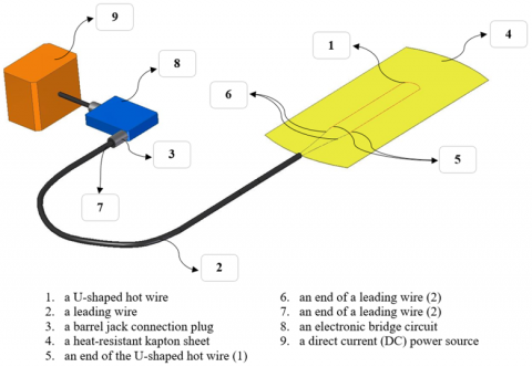
This study aims to utilize the dynamic hot-wire method, which operates on transient principles, to determine the thermal conductivity of liquid substances, encompassing both electrically conductive and non-conductive samples. As illustrated in Figure 1, an experimental apparatus for measuring thermal conductivity consists of a sensor unit, an electronic bridge circuit in electrical communication with the sensor unit, and a DC power source in electrical communication with the electronic bridge circuit.
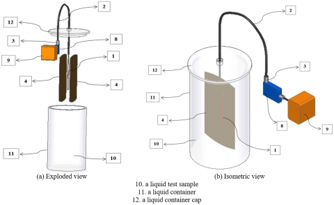
3.1 Sensor unit
A novel apparatus for determining thermal conductivity was developed by incorporating a sensor unit, as illustrated in Figure 1, labelled as 1 to 7 in the sensor unit. This sensor unit consists of a U-shaped hot-wire, a leading wire, a barrel jack plug, and two heat-resistant sheets that encapsulate the U-shaped hot-wire.
Figure 1. Experimental apparatus
3.1.1 U-shaped hot-wire
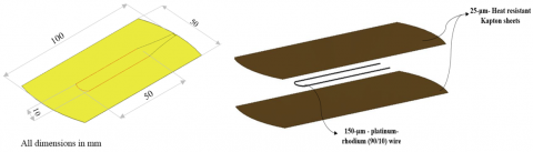
A U-shaped hot-wire comprising a platinum-rhodium alloy (90% platinum, 10% rhodium) wire with a length of 100 mm and a cross-sectional diameter of 150 μm was utilized. This electrically resistive material is configured in a U-shaped geometry, which enhances its applicability to various industrial, scientific, and monitoring applications. The U-shaped design improves the sensitivity, adaptability, and spatial resolution of hot-wire sensors. In addition to functioning as a temperature sensor that detects resistance fluctuations, the U-shaped hot-wire also serves as a heating element when immersed in the liquid test samples. This dual functionality generated a time-varying temperature field within the liquid sample. The configuration of the U-shaped wire encased between two heat-resistant Kapton sheets is illustrated in Figure 2.
Figure 2. Geometry of a U-shaped hot-wire laminated using two heat-resistant sheets
3.1.2 Leading wire
The lead wire is a low-noise, twin-core 0.5 mm diameter cable with shielding. At one end of the lead wire, the point at which it connects to the hot-wire was a spot weld. The other end of the lead has a barrel connector. The lead not only connects to the sensor but also supports the U-shape of the sensor. This design created no mechanical stress on the U-shaped hot-wire when connecting or disconnecting the hot-wire sensor from an electrical source. The use of a spot-welding method to join the lead wire and U-shaped hot-wire created a secure, low impedance connection between them.
3.1.3 Barrel jack plug
The barrel jack connector (also referred to as the coaxial power connector) is a cylindrical electrical connector commonly used to supply low-voltage DC power to electronic devices. The plug consists of a 2 mm inner pin and a 6 mm outer sleeve, which provides the means for proper power and polarity transfer. Barrel jack connectors create a secure electrical contact for reliable connection; this feature is particularly valuable with associated locking connectors for stabilizing equipment positioned in locations exposed to vibration.
3.1.4 Heat-resistant sheets
Heat-resistant sheets, such as Kapton, exhibit exceptional thermal stability (-269℃ to 260℃) and mechanical properties. The remarkable combination of electrical insulation, chemical resistance, and dimensional stability makes it highly suitable for applications that require elevated temperatures. To protect the U-shaped hot-wire, provide electrical insulation, and mitigate polarization effects on the wire surface, it was encapsulated between two heat-resistant sheets (25 μm thick, 100 mm long, and 50 mm wide).
3.2 Electronic components
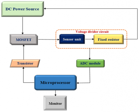
The electronic bridge circuit investigated in this research is depicted in Figure 3. The electronic bridge circuit consists of a D.C. power supply connected to a voltage divider circuit; an Analog to digital converter (ADC) module connecting into the voltage divider circuit; a MOSFET switch that provides the voltage measurement through the voltage divider circuit; a transistor controlling the MOSFET switch and a microprocessor connected to the ADC module and to the transistor controlling the MOSFET switch.
Figure 3. Electronic bridge circuit
3.2.1 Voltage divider circuit
The sensor unit was connected, in series, to a 0.5-ohm fixed resistor as part of the resistor-divider (voltage divider) circuit. The resistor-divider circuit divides the input voltage produced by the DC supply into several smaller voltages.
The output from the circuit, where the platinum/rhodium wire meets the 0.5-ohm fixed resistor, is measured as the voltage drop across the fixed resistor. By measuring the voltage, we can determine the resistance of the platinum/rhodium wire using Ohm's law based on the value of the fixed resistor and the value of the measured voltage. The resistance of the platinum/rhodium wire can then be converted into a corresponding temperature reading. This can be accomplished using the Callendar-Van Dusen equation, which provides a mathematical relationship for converting resistance readings to temperature values.
3.2.2 Direct current power source
During the test procedure, the sensor unit received a DC power source. This supply maintained a continuous electrical current flow to the circuit at a regulated level. The regulated power supply has maximum settings for voltage (30 V) and current (2 A). Upon reaching the high demand level for current in the electronic bridge circuit, the regulated power supply will quickly enter into constant current mode via the use of an internal voltage to constant current transition circuit that can operate at a 0.5-ohm fixed resistor load and U-shaped hot-wire resistance in about 1 millisecond following an applied voltage set point. The constant current mode is used for stabilizing the temperature of hot-wire sensors.
3.2.3 Analog to digital converter module
The ADC is a key element in many electronics applications by interfacing the analog and digital domains. It takes the voltage level from an analog sensor as input and converts it to a digital output in discrete steps based on the ADC's conversion rate and time frame. In the present work, the sensor connects to the ADC via a 0.5 Ω fixed resistor. The ADS1115 is a 16-bit, up to 860 samples per second (S/s) ADC. A "16-bit" ADC means the ADC can distinguish 65536 separate voltage readings (0 through 65535). Since the ADS1115 can also measure negative voltages, the ADC is set to read values in the range of -32768 to 32768. The way we determine the actual voltage measurement is by comparing the range of values that the ADC produces to a voltage range of -3.3 V to 3.3 V. The final computation is done using a Python script running on a Raspberry Pi. The ADS1115 uses the Serial Peripheral Interface (SPI) protocol as its means of communicating with the Raspberry Pi, which allows for real-time, two-way communication.
3.2.4 Transistors and MOSFETs
Modern electronic devices depend heavily on transistors and MOSFETs, which function as both switches and amplifiers in a wide array of applications. Acting as an interface, the transistor bridges the gap between the MOSFET switch, which operates on 5 V logic, and the Raspberry Pi's GPIO pins, which produce a 3.3 V signal. The Raspberry Pi regulates the transistor via GPIO 4. To activate the transistor, a minimum current must flow from its base to the emitter, which is controlled by a 1-kiloohm resistor. The MOSFET switch is active-low, indicating that it is activated when GPIO 4 is LOW and deactivated when GPIO 4 is HIGH. In the Raspberry Pi terminology, LOW corresponds to 0 V and HIGH to 3.3 V. The MOSFET switch requires 5 V at its gate to turn ON and 0 V to turn OFF. When GPIO 4 is HIGH, the transistor conducts, reducing the gate of the MOSFET switch to 0 V and deactivating it. Conversely, when GPIO 4 is LOW, the transistor is OFF, allowing the gate voltage to increase to 5 V due to a 10-kiloohm pull-up resistor, thereby activating the MOSFET switch. To maintain the MOSFET switch in the OFF state by default, GPIO 4 transmits a HIGH signal. GPIO 4 was set to LOW only when the measurements commenced.
3.2.5 Raspberry Pi – microprocessor
Raspberry Pi is a compact single-board computer comprising a 64-bit Broadcom BCM2837 chip with four cores operating at 1.2 GHz and 1 GB of RAM. This miniature computer operates on the Raspbian OS, which is stored on a 16 GB SD card. The device is equipped with USB and HDMI ports as well as 40 GPIO pins to facilitate the connection of various hardware components. It requires a 5.1 V 3 A power supply for operation. The Raspberry Pi can be used as a mini PC by connecting a mouse, keyboard, and monitor to their corresponding ports. It can also be used for writing and running Python programs directly on the Raspberry Pi. A Python program that runs on the Raspberry Pi triggers a resistor divider circuit through a MOSFET switch to collect analog data with the help of an ADC module. The application software program produces a CSV file with temperature and time data. A temperature vs. time graph formed from the temperature/time data shows the thermal conductivity of the liquid sample. The thermal conductivity value can be calculated from the slope (gradient) of the straight line (linear) portion of the temperature vs. time graph.
3.3 Sources of the test samples
It is essential to provide information about the sources of test samples to ensure the reproducibility and reliability of scientific research. This includes specifying the origin, collection methods, and any relevant characteristics of the samples used in the present study.
(i) The engine oil sample used in this study was a commercially available SAE 5W-30 multigrade oil (Brand: Castrol synthetic, in Mysore, India). The oil met the specifications of SN, SP, and ILSAC GF-6A or GF-6B standards.
(ii) The water sample used in experiments was obtained from an in-house Aquaguard water purification system (Aquaguard Glory, resistivity ≥ 18.2 MΩ·cm, pH = 7.0 (neutral), at 25 ℃).
(iii) The new commercial-grade mineral-based transformer oil sample used in this study was obtained from Karnataka Power Transmission Corporation Limited (KPTCL) and was compliant with the Bureau of Indian Standards (BIS) specifications for electrical insulation and thermal performance.
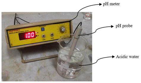
(iv) The acidic water (pH = 1) sample used in the present study was freshly prepared in the laboratory. When preparing acidic water, a strong acid, such as hydrochloric acid (HCl), is selected. A small volume of the concentrated acid was measured and slowly added to a larger volume of water while stirring gently. The pH of the resulting solutions was then tested using a pH meter or indicator, as shown in Figure 4 (0.1 M HCl solution from a 12 M stock, 2.5 mL of the concentrated acid is diluted with 297.5 mL of water, yielding 300 mL of solution with a pH of approximately 1).
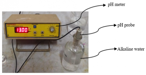
(v) The alkaline water (pH = 13) sample used in the present study was freshly prepared in the laboratory. To prepare alkaline water, a strong base such as sodium hydroxide (NaOH) was used. A small quantity of the base was measured and gradually added to a larger volume of water with careful mixing. The pH of the sample was subsequently determined utilizing a pH probe, as illustrated in Figure 5 (dissolving 1.2 grams of NaOH pellets in water and diluting to a total volume of 300 mL results in a 0.1 M NaOH solution with a pH around 13).
Figure 4. Measurement of acidic water using a digital pH meter
Figure 5. Measurement of alkaline water using a digital pH meter
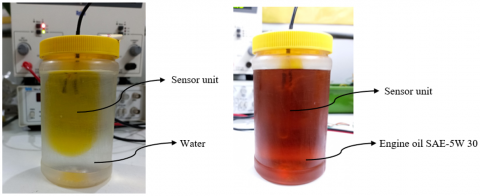
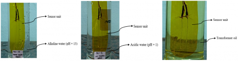
The present study utilized an apparatus and methodology to measure the thermal conductivity of liquid specimens, including water, SAE-5W-30 engine oil, alkaline water (pH = 13), acidic water (pH = 1), and transformer oil. To conduct the measurements, a U-shaped hot-wire laminated with a heat-resistant sheet was fully immersed in the liquid test sample. This configuration facilitates efficient thermal conduction from the U-shaped hot-wire through the heat-resistant sheet to the liquid under investigation. Figure 6 illustrates the arrangement of the U-shaped wire with its heat-resistant sheet and the liquid sample, which was utilized to measure the thermal conductivity under ambient conditions. A photographic representation of the apparatus submerged in the liquid test sample for thermal conductivity measurements is shown in Figure 7.
To ensure that the physical system is operating within the acceptable limits, it is critical that the t1 and t2 measurement cycle duration be the optimal choice. From the experimental results, it can be seen that a heat pulse, or heat signature, with a duration of approximately 1 second and delivered via U-shaped hot-wire to the liquid sample through a heat-resistant sheet allows enough time for the temperature to increase between t1 and t2 with an input power level of approximately 3 W. During the testing, there were 300 measurements collected within the time frame of 0 to 1 seconds. The choice of using a 3 W input power level within the transient hot-wire method is dependent on several important elements for obtaining accurate thermal conductivity measurements. The use of the 3 W input level results in a significantly observable increase in temperature (approximately 2 to 5 K) in the hot-wire between times t1 and t2, while not producing excessive heat that could produce an effect on the material properties or result in unwanted convection [42-44]. Additionally, the 3 W power input level produces minimal electronic noise, which provides assurance of measurement stability, and this also leads to an increased ability to measure the temperature rise accurately [45]. Furthermore, the consistent power input of 3 W allows for model calibration and validation against the corresponding established standards.
Thermal conductivity measurements encompassed three distinct phases. Initially, experimental resistance measurements were obtained from a U-shaped hot-wire over a predetermined time interval. In turn, the temperature data was calculated based on these measurements. Over time, the temperature of the U-shaped hot-wire follows a logarithmic trend. Thus, in order to determine the thermal conductivities from the temperature curve obtained by plotting temperature versus time using the transient hot-wire technique on a semi-logarithmic scale, it is customary to omit the initial portion of the temperature/time data points [46]. Therefore, our analysis focuses on the upper linear segment of the graph. This methodology is essential for obtaining precise thermal conductivity measurements and involves several critical factors. The initial portion of the temperature-time graph frequently exhibits transient effects that do not conform to the steady-state heat conduction model. During this phase, the temperature increase may be influenced by thermal inertia and other transient phenomena, which can potentially distort measurements [46]. The upper linear portion of the graph indicates the establishment of a quasi-steady-state or thermal equilibrium in which temperature increases have been observed to continue on a consistent and expected basis. This linear behaviour demonstrates that the system had been brought to a point where the assumptions made in the transient hot-wire model are valid, and thus thermal conductivity may be accurately determined from the slope of the line [46]. By concentrating on the linear segment, the impact of noise and irregularities present in the initial transient phase can be minimized, thereby enhancing the measurement accuracy, as data points from the steady linear segment are less susceptible to such disturbances.
The use of a semi-logarithmic scale facilitates the clear identification of the linear segment, thereby simplifying the derivation of the thermal properties by converting the exponential temperature increase into a linear form. This transformation is crucial for aligning the observed temperature increase with the theoretical model, enabling the determination of the thermal conductivity [46]. The use of these methods allows for taking the data used for determining thermal conductivity from a relatively wide range in which all mechanisms of heat transfer are assumed to be known and accurately modeled by theoretical models used in the analysis. From the initial portion of the data to the linear portion, the errors in thermal conductivity values were reduced significantly. Thus, as a result, thermal conductivity values were less prone to error and therefore more reliable.
Figure 6. Arrangement of an apparatus for measuring the thermal conductivity of a liquid test sample
Figure 7. Photograph showing a device as per the present work immersed in a liquid test sample for the measurement of thermal conductivity of water and SAE-5W-30 engine oil
The selection of the upper linear segment is based on the observation that, during this phase, the increase in the wire temperature exhibits a direct linear correlation with the natural logarithm of time. The correlation observed occurs because of a predominance of conduction occurring over this time frame with little interference from any other type of heat transfer (e.g., convection). The linear relationship observed during this region occurred as a result of having sufficient data points to produce a linear plot with little deviation, validating that the primary cause of heat transfer in this region occurs from conduction [47]. To achieve a more precise quantification of the deviation in the linear segment, we employed Linear Regression Analysis. It is beneficial if the R-squared value of the linear fit approaches 1, indicating a strong linear relationship, and if the selected region yields consistent results across multiple measurements of the same sample.
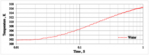
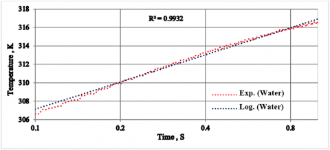
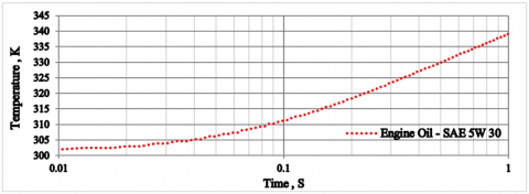
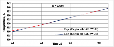
The empirical results depicting the relationship between the temperature and time for water and SAE-5W-30 engine oil are presented in semi-logarithmic plots in Figures 8 and 9. These data were collected at ambient temperature using the equipment developed in this study. The thermal conductivities of the liquid samples were determined from the upper linear portion of the curve. For measurement purposes, 0.1 seconds is designated as t1 and 1 second as t2. The calculated thermal conductivity values for water and engine oil SAE-5W 30 derived from these semi-logarithmic temperature-time plots are 0.58 W/m·K and 0.131 W/m·K, respectively. These results deviate from those proposed in the literature by -0.02 to -0.03 and -0.005, respectively [48-50].
Tables 1 and 2 show an evaluation of assessed thermal conductivity and its deviations for liquid test samples employing the present developed apparatus and the value suggested by the literature [48-50].
(a)
(b)
Figure 8. (a) An experimental temperature v/s time curve for water and (b) its Logarithmic Fit for the linear portion of the experimental data
(a)
(b)
Figure 9. (a) An experimental temperature v/s time curve for SAE-5W-30 engine oil and (b) its Logarithmic Fit for the linear portion of the experimental data
Table 1. Evaluation of assessed thermal conductivity and its deviations for the water test sample and the value suggested by the literature
|
Electrically Conductive Liquid Sample - Water |
||||
|
Trial No. |
Measured Thermal Conductivity (W/m·K) at 300 K |
Literature [48] Thermal Conductivity (W/m·K) at 300 K |
Literature [49] Thermal Conductivity (W/m·K) at 300 K |
Deviations |
|
1 |
0.58 |
0.60 |
0.61 |
-0.02 [48] -0.03 [49] |
|
2 |
0.57 |
|||
|
3 |
0.59 |
|||
|
Mean |
0.58 |
|||
|
Standard deviation |
0.016 |
|
|
|
|
Random uncertainty (from repeated measurements) (%) |
2.72% |
|
|
|
Table 2. Evaluation of assessed thermal conductivity and its deviations for the SAE-5W-30 engine oil test sample and the value suggested by the literature
|
Electrically Non-Conductive Liquid Sample - SAE-5W-30 Engine Oil |
|||
|
Trial No. |
Measured Thermal Conductivity (W/m·K) at 300 K |
Literature [50] Thermal Conductivity (W/m·K) at 300 K |
Deviations |
|
1 |
0.131 |
0.136 |
-0.005 [50] |
|
2 |
0.129 |
||
|
3 |
0.133 |
||
|
Mean |
0.131 |
||
|
Standard deviation |
0.002 |
|
|
|
Random uncertainty (from repeated measurements) (%) |
1.53% |
|
|
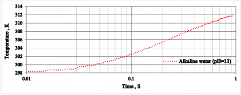
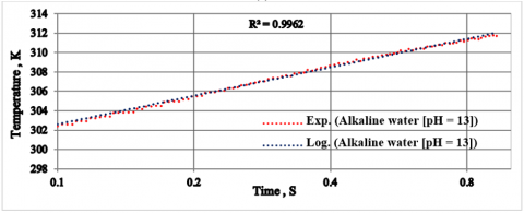
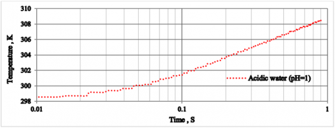
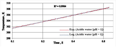
To evaluate the broad applicability of the developed device, it is imperative to incorporate liquid samples from diverse sources. By assessing the device across various liquid samples, researchers can ascertain its performance in different contexts and identify any limitations or areas for improvement. The thermal conductivities of several liquids were examined in the present study: highly acidic water (pH = 1) and highly alkaline water (pH = 13), which represent electrically conductive liquids, and transformer oil, which represents electrically nonconductive liquids. Figure 10 shows a photographic depiction of the apparatus immersed in the sample for measuring thermal conductivity. Figures 11, 12, and 13 show semi-logarithmic graphs depicting the correlations between the temperature and time for the alkaline water, acidic water, and transformer oil. These findings were obtained at ambient temperature using the apparatus developed in this study.
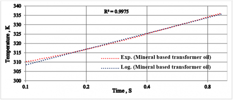
The thermal conductivities of alkaline water, acidic water, and transformer oil, as determined from the semi-logarithmic temperature-time graphs, were 0.59, 0.63, and 0.148 W/m·K, respectively. These findings showed variations from the literature by -0.02 for alkaline, +0.02 for acidic water, and +0.018 for transformer oil [49, 51].
Tables 3, 4, and 5 provide an evaluation of the measured thermal conductivities and their deviations for the test samples using the developed apparatus, in comparison with the literature values [49, 51].
Figure 10. Photograph showing a device as per the present work immersed in a liquid test sample for the measurement of thermal conductivity of alkaline water, acidic water, and transformer oil
(a)
(b)
Figure 11. (a) An experimental temperature v/s time curve for alkaline water and (b) its Logarithmic Fit for the linear portion of the experimental data
(a)
(b)
Figure 12. (a) An experimental temperature v/s time curve for acidic water and (b) its Logarithmic Fit for the linear portion of the experimental data
(a)
(b)
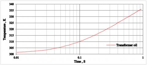
Figure 13. (a) An experimental temperature v/s time curve for mineral-based transformer oil and (b) its Logarithmic Fit for the linear portion of the experimental data
Table 3. Evaluation of assessed thermal conductivity and its deviations for alkaline water
|
Electrically Conductive Liquid Sample - Alkaline Water [pH = 13] |
|||
|
Trial No. |
Measured Thermal Conductivity (W/m·K) at 300 K |
Literature [49] Thermal Conductivity (W/m·K) at 300 K |
Deviations |
|
1 |
0.58 |
0.61 |
-0.02 [49] |
|
2 |
0.60 |
||
|
3 |
0.59 |
||
|
Mean |
0.59 |
||
|
Standard deviation |
0.01 |
|
|
|
Random uncertainty (from repeated measurements) (%) |
1.6% |
|
|
Table 4. Evaluation of assessed thermal conductivity and its deviations for acidic water
|
Electrically Conductive Liquid Sample - Acidic Water [pH = 1] |
|||
|
Trial No. |
Measured Thermal Conductivity (W/m·K) at 300 K |
Literature [49] Thermal Conductivity (W/m·K) at 300 K |
Deviations |
|
1 |
0.61 |
0.61 |
+0.02 [49] |
|
2 |
0.63 |
||
|
3 |
0.65 |
||
|
Mean |
0.63 |
||
|
Standard deviation |
0.028 |
|
|
|
Random uncertainty (from repeated measurements) (%) |
4.44% |
|
|
Table 5. Evaluation of assessed thermal conductivity and its deviations for transformer oil
|
Electrically Non-Conductive Liquid Sample - Mineral-Based Transformer Oil |
|||
|
Trial No. |
Measured Thermal Conductivity (W/m·K) at 300 K |
Literature [51] Thermal Conductivity (W/m·K) at 300 K |
Deviations |
|
1 |
0.152 |
0.130 |
+0.018 [51] |
|
2 |
0.145 |
||
|
3 |
0.147 |
||
|
Mean |
0.148 |
||
|
Standard deviation |
0.004 |
|
|
|
Random uncertainty (from repeated measurements) (%) |
2.43% |
|
|
The pH level influences the concentration of ions in water, thereby affecting electrical conductivity. However, this had a minimal impact on the thermal conductivity. The primary mechanism of heat transfer in water is molecular vibration and collision, which remains largely unaffected by ion concentration. Consequently, the thermal conductivities of both alkaline and acidic waters were nearly equivalent to that of pure water [52, 53].
Potential reasons for the discrepancies between the measured thermal conductivity values and those reported in the literature include inherent measurement uncertainties. The developed device exhibited a standard uncertainty of ±2.4% (as described in the following section), which may partially account for the observed differences. Variations in the experimental setup, including differences in sensor design, such as the use of a U-shaped platinum-rhodium wire versus traditional straight wires, wire geometry, material properties, and insulation with Kapton sheets, can influence the heat transfer characteristics and measurement accuracy. Sample purity and preparation also play a role, as impurities, exact pH values, and temperature during the measurement may differ from the reference conditions. Environmental factors, such as ambient temperature fluctuations and convection currents, can affect readings. The variation of the calibration and reference standard in this study, compared to other literature sources, may cause a slight shift in the reported value. The thermal conductivity of a liquid can differ based on the composition of the liquid, i.e., the presence of ions/additives.
The novel device and methodology are appropriate for determining the thermal conductivity of both electrically conductive and non-conductive liquid samples under transient conditions. The measurement requires only 1 s, facilitating a more rapid evaluation compared to the existing methods. Furthermore, this innovative approach provides a straightforward, efficacious, and cost-effective alternative to the current techniques.
4.1 Uncertainty analysis for the thermal conductivity measurements
The guidelines for assessing uncertainty, formally termed the Guide to the Uncertainty of Measurement and released by the International Organization for Standardization (ISO), were applied [54]. The influence of the factors on the standard uncertainty is depicted in Eq. (13).
$\left(\frac{u(k)}{k}\right)^2=\left(\frac{u(V)}{V}\right)^2+\left(\frac{u(s)}{s}\right)^2+\left(\frac{u(t)}{t}\right)^2+\left(\frac{u(Q)}{Q}\right)^2+\left(\frac{u(B)}{B}\right)^2$ (13)
The standard uncertainty in the thermal conductivity is denoted as u(V), u(S), u(t), u(Q), and u(B) represent the standard uncertainties associated with the voltage source applied to the voltage divider circuit, the wire temperature fluctuation to log base e slope fit, the experiment time, the heat emitted per unit span of the hot-wire, and the thermal coefficient of the hot-wire, respectively.
In the present work, the standard uncertainty in the thermal conductivity of the liquids was assessed as follows. An electronic fine-precision multimeter with an uncertainty of ±1 μV was used to monitor the potential difference supplied to the voltage divider circuit and its variations during a transient test, and the fluctuation in the wire temperature with respect to the log base e of time was recorded with an uncertainty of ±2%, as determined by nonlinear discrepancies. The experimental time was measured and registered using an ADC (ADS1115) with a 16-bit conversion, a maximum data rate of 860 samples per second, and an uncertainty of ±1 μs. An uncertainty of ±0.2% was determined for the heat produced per unit of length using a platinum-rhodium wire made up of 90% Platinum and 10% Rhodium. The uncertainty in measuring the thermal coefficient of resistance of a thin platinum-rhodium wire when using a calibrated technique to assess the thermal coefficient of resistance was found to be ±0.2%. The test sensor device was constructed with layers of 50 μm thick Kapton heat-resistant sheets with proven tolerances, eliminating any influence on the uncertainty of this method; hence, the developed device was determined to have a standard uncertainty of ±2.4% when measuring the thermal conductivity of liquids.
In this study, a novel transient hot-wire apparatus was developed and validated for the accurate measurement of the thermal conductivity of both electrically conductive and nonconductive liquids within a rapid timeframe of one second. By employing a U-shaped platinum-rhodium wire sensor encapsulated in heat-resistant Kapton sheets, the device demonstrated operational simplicity, cost-effectiveness, and enhanced measurement precision compared with existing methods. The experimental results for various liquid samples, including water, SAE-5W-30 engine oil, alkaline water (pH = 13), acidic water (pH = 1), and transformer oil, were in close agreement with previously reported data. The thermal conductivities measured were 0.58, 0.313, 0.59, 0.63, and 0.148 W/m·K for water, SAE-5W-30 engine oil, alkaline water, acidic water, and transformer oil, respectively. The standard uncertainty of the developed instrument was ±2.4%. The ability of the apparatus to deliver fast and reliable measurements makes it particularly suitable for real-time thermal management applications in the electronics, automotive, energy storage, chemical processing, and HVAC industries.
The primary contributions of this work include the design of a versatile sensor unit that overcomes the limitations of traditional transient hot-wire methods, such as insulation-related measurement errors and long test durations, and the integration of a custom electronic bridge circuit and data acquisition system for precise temperature monitoring. This integration enables rapid, stable, and reproducible thermal conductivity measurements, irrespective of the electrical conductivity of the liquid sample. Perspective research should focus on optimizing sensor performance by exploring alternative wire materials and geometries to broaden the measurable liquid range and improve the sensitivity. Extending the operational envelope of the apparatus to cover wider temperature and pressure ranges. Implementing these enhancements will solidify the utility of the device as a standard instrument for fast and accurate thermal conductivity characterization in both research and industrial settings.
The authors acknowledge JSS Science and Technology University, Mysore, Karnataka, India / National Institute of Technology, Karnataka, Surathkal, Mangalore, India, for providing the necessary facilities to conduct this work.
|
cp |
specific heat in J/kg K |
|
r |
radius of the wire in m |
|
T |
temperature in kelvin |
|
t |
time in seconds |
|
k |
thermal conductivity in W/m·K |
|
q |
heat flux per unit length or Power input per unit distance in W/m |
|
ln t |
logarithm of time in seconds |
|
Greek symbols |
|
|
ρ |
density in kg/m3 |
|
∆T |
temperature rise in kelvin |
[1] Eastman, J.A., Choi, S.U.S., Li, S., Yu, W., Thompson, L.J. (2001). Anomalously increased effective thermal conductivities of ethylene glycol-based nanofluids containing copper nanoparticles. Applied Physics Letters, 78(6): 718-720. https://doi.org/10.1063/1.1341218
[2] Huminic, G., Huminic, A. (2012). Application of nanofluids in heat exchangers: A review. Renewable and Sustainable Energy Reviews, 16(8): 5625-5638. https://doi.org/10.1016/j.rser.2012.05.023
[3] Sundar, L.S., Singh, M.K., Sousa, A.C.M. (2014). Enhanced heat transfer and friction factor of MWCNT-Fe3O4/water hybrid nanofluids. International Communications in Heat and Mass Transfer, 52: 73-83. https://doi.org/10.1016/j.icheatmasstransfer.2014.01.012
[4] Turgut, A., Tavman, I., Tavman, S. (2009). Measurement of thermal conductivity of edible oils using transient hot wire method. International Journal of Food Properties, 12(4): 741-747. https://doi.org/10.1080/10942910802023242
[5] Hoffmann, J.F., Henry, J.F., Vaitilingom, G., Olives, R., Chirtoc, M., Caron, D., Py, X. (2016). Temperature dependence of thermal conductivity of vegetable oils for use in concentrated solar power plants, measured by 3omega hot wire method. International Journal of Thermal Sciences, 107: 105-110. https://doi.org/10.1016/j.ijthermalsci.2016.04.002
[6] Wang, H.J., Ma, S.J., Yu, H.M., Zhang, Q., Guo, C.M., Wang, P. (2014). Thermal conductivity of transformer oil from 253 K to 363 K. Petroleum Science and Technology, 32(17): 2143-2150. https://doi.org/10.1080/10916466.2012.757235
[7] Elam, S.K., Tokura, I., Saito, K., Altenkirch, R.A. (1989). Thermal conductivity of crude oils. Experimental Thermal and Fluid Science, 2(1): 1-6. https://doi.org/10.1016/0894-1777(89)90043-5
[8] Jagueneau, A., Jannot, Y., Degiovanni, A., Ding, T. (2019). A steady-state method for the estimation of the thermal conductivity of a wire. International Journal of Heat and Technology, 37(1): 351-356. https://doi.org/10.18280/ijht.370142
[9] Yassien, H.N.S., Mustafa, A.O.A., Soheel, A.H., Hassan, F.I.A. (2023). Experimental investigation on the effect of sawdust particles size on its thermal conductivity. International Journal of Heat and Technology, 41(2): 475-480. https://doi.org/10.18280/ijht.410224
[10] Holeschovsky, U.B., Martin, G.T., Tester, J.W. (1996). A transient spherical source method to determine thermal conductivity of liquids and gels. International Journal of Heat and Mass Transfer, 39(6): 1135-1140. https://doi.org/10.1016/0017-9310(95)00210-3
[11] Omotani, T., Nagasaka, Y., Nagashima, A. (1982). Measurement of the thermal conductivity of KNO3-NaNO3 mixtures using a transient hot-wire method with a liquid metal in a capillary probe. International Journal of Thermophysics, 3(1): 17-26. https://doi.org/10.1007/BF00503955
[12] Perkins, R.A., Roder, H.M., Nieto de Castro, C.A. (1991). High-temperature transient hot-wire thermal conductivity apparatus for fluids. Journal of Research of the National Institute of Standards and Technology, 96(3): 247-269. https://doi.org/10.6028/jres.096.014
[13] Campagnoli, E., Valter, V. (2020). Experimental investigation on thermal conductivity and thermal diffusivity of water-agar gel from room temperature to -60 ℃. International Journal of Heat and Technology, 38(3): 583-589. https://doi.org/10.18280/ijht.380302
[14] Ai, Q., Hu, Z.W., Wu, L.L., Sun, F.X., Xie, M. (2017). A single-sided method based on transient plane source technique for thermal conductivity measurement of liquids. International Journal of Heat and Mass Transfer, 109: 1181-1190. https://doi.org/10.1016/j.ijheatmasstransfer.2017.03.008
[15] Hoque, M.S.B., Ansari, N., Khodadadi, J.M. (2018). Explaining the “anomalous” transient hot wire-based thermal conductivity measurements near solid-liquid phase change in terms of solid-solid transition. International Journal of Heat and Mass Transfer, 125: 210-217. https://doi.org/10.1016/j.ijheatmasstransfer.2018.04.014
[16] Carslaw, H.S., Jaeger, J.C. (1948). Conduction of Heat in Solids (2nd ed.). Oxford University Press.
[17] Liang, X., Ding, W., Shu, Z., Zhou, X., Gao, D. (2008). A micromachined device using transient hot-wire method for high accuracy thermal conductivity measurement of semi-rigid materials. In Proceedings of the 3rd Frontiers in Biomedical Devices Conference and Exhibition, pp. 71-72. https://doi.org/10.1115/biomed2008-38038
[18] Azarfar, S., Movahedirad, S., Sarbanha, A.A., Norouzbeigi, R., Beigzadeh, B. (2016). Low cost and new design of transient hot-wire technique for the thermal conductivity measurement of fluids. Applied Thermal Engineering, 105: 142-150. https://doi.org/10.1016/j.applthermaleng.2016.05.138
[19] Gross, U., Song, Y.W., Hahne, E. (1992). Measurements of liquid thermal conductivity and diffusivity by the transient hot-strip method. Fluid Phase Equilibria, 76: 273-282. https://doi.org/10.1016/0378-3812(92)85094-O
[20] Tian, F., Sun, L., Mojumdar, S.C., Venart, J.E.S., Prasad, R.C. (2011). Absolute measurement of thermal conductivity of polyacrylic acid by transient hot wire technique. Journal of Thermal Analysis and Calorimetry, 104(3): 823-829. https://doi.org/10.1007/s10973-010-1261-3
[21] Nakamura, S., Hibiya, T., Yamamoto, F. (1988). New sensor for measuring thermal conductivity in liquid metal by transient hot wire method. Review of Scientific Instruments, 59(6): 997-998. https://doi.org/10.1063/1.1139771
[22] Watanabe, H. (1996). Accurate and simultaneous measurement of the thermal conductivity and thermal diffusivity of liquids using the transient hot-wire method. Metrologia, 33(2): 101-115. https://doi.org/10.1088/0026-1394/33/2/1
[23] Kwon, S.Y., Lee, S. (2012). Precise measurement of thermal conductivity of liquid over a wide temperature range using a transient hot-wire technique by uncertainty analysis. Thermochimica Acta, 542: 18-23. https://doi.org/10.1016/j.tca.2011.12.015
[24] Stanimirović, A.M., Živković, E.M., Milošević, N.D., Kijevčanin, M.L. (2017). Application and testing of a new simple experimental set-up for thermal conductivity measurements of liquids. Thermal Science, 21(3): 1195-1202. https://doi.org/10.2298/TSCI160324219S
[25] Fox, J.N., Gaggini, N.W., Wangsani, R. (1987). Measurement of the thermal conductivity of liquids using a transient hot wire technique. American Journal of Physics, 55(3): 272-274. https://doi.org/10.1119/1.15177
[26] Tian, F., Sun, L., Venart, J.E.S., Prasad, R.C. (2009). Thermal conductivity and thermal diffusivity of polyacrylic acid by transient hot wire technique: Absolute measurement. Journal of Thermal Analysis and Calorimetry, 96(1): 67-71. https://doi.org/10.1007/s10973-008-9840-2
[27] Calado, J.C.G., Mardolcar, U.V., de Castro, C.N., Roder, H.M., Wakeham, W.A. (1987). The thermal conductivity of liquid argon. Physica A: Statistical Mechanics and its Applications, 143(1-2): 314-325. https://doi.org/10.1016/0378-4371(87)90071-9
[28] Tuliszka, M., Jaroszyk, F., Portalski, M. (1991). Absolute measurement of the thermal conductivity of propylene carbonate by the AC transient hot-wire technique. International Journal of Thermophysics, 12(5): 791-800. https://doi.org/10.1007/BF00502406
[29] Nieto de Castro, C.A., Perkins, R.A., Roder, H.M. (1991). Radiative heat transfer in transient hot-wire measurements of thermal conductivity. International Journal of Thermophysics, 12(6): 985-997. https://doi.org/10.1007/BF00503514
[30] Garnier, J.P., Maye, J.P., Saillard, J., Thévenot, G., Kadjo, A., Martemianov, S. (2008). A new transient hot-wire instrument for measuring the thermal conductivity of electrically conducting and highly corrosive liquids using small samples. International Journal of Thermophysics, 29(2): 468-482. https://doi.org/10.1007/s10765-008-0388-y
[31] Guo, W., Li, G., Zheng, Y., Dong, C. (2018). Measurement of the thermal conductivity of SiO2 nanofluids with an optimized transient hot wire method. Thermochimica Acta, 661: 84-97. https://doi.org/10.1016/j.tca.2018.01.008
[32] Kitazawa, N., Nagashima, A. (1981). Measurement of thermal conductivity of liquids by a transient hot-wire method: II, measurement under high pressure. Bulletin of JSME, 24(188): 374-379. https://doi.org/10.1299/jsme1958.24.374
[33] Alloush, A., Gosney, W.B., Wakeham, W.A. (1982). A transient hot-wire instrument for thermal conductivity measurements in electrically conducting liquids at elevated temperatures. International Journal of Thermophysics, 3(3): 225-235. https://doi.org/10.1007/BF00503318
[34] Cohen, E., Glicksman, L. (2014). Analysis of the transient hot-wire method to measure thermal conductivity of silica aerogel: Influence of wire length, and radiation properties. Journal of Heat Transfer, 136(4): 1-8. https://doi.org/10.1115/1.4025921
[35] Antoniadis, K.D., Tertsinidou, G.J., Assael, M.J., Wakeham, W.A. (2016). Necessary conditions for accurate, transient hot-wire measurements of the apparent thermal conductivity of nanofluids are seldom satisfied. International Journal of Thermophysics, 37(8): 78. https://doi.org/10.1007/s10765-016-2083-8
[36] Woodfield, P.L., Fukai, J., Fujii, M., Takata, Y., Shinzato, K. (2008). A two-dimensional analytical solution for the transient short-hot-wire method. International Journal of Thermophysics, 29(4): 1278-1298. https://doi.org/10.1007/s10765-008-0469-y
[37] Nieto de Castro, C.A., Wakeham, W.A. (1978). Experimental aspects of the transient hot-wire technique for thermal conductivity measurements. In Thermal Conductivity 15, pp. 235-243. https://doi.org/10.1007/978-1-4615-9083-5_30
[38] Bran-Anleu, G., Lavine, A.S., Wirz, R.E., Kavehpour, H.P. (2014). Algorithm to optimize transient hot-wire thermal property measurement. Review of Scientific Instruments, 85(4): 045105. https://doi.org/10.1063/1.4870275
[39] Healy, J.J., De Groot, J.J., Kestin, J. (1976). The theory of the transient hot-wire method for measuring thermal conductivity. Physica B+ c, 82(2): 392-408. https://doi.org/10.1016/0378-4363(76)90203-5
[40] Assael, M.J., Antoniadis, K.D., Wakeham, W.A. (2010). Historical evolution of the transient hot-wire technique. International Journal of Thermophysics, 31(6): 1051-1072. https://doi.org/10.1007/s10765-010-0814-9
[41] Babu, S.K., Praveen, K.S., Raja, B., Damodharan, P. (2013). Measurement of thermal conductivity of fluid using single and dual wire transient techniques. Measurement, 46(8): 2746-2752. https://doi.org/10.1016/j.measurement.2013.05.017
[42] ISO, E. (2010). 8894-1: Refractory materials: Determination of thermal conductivity-part1: Hot-wire methods (cross-array and resistance thermometer). Matériaux réfractaires.
[43] Assael, M.J., Gialou, K., Kakosimos, K., Metaxa, I. (2004). Thermal conductivity of reference solid materials. International Journal of Thermophysics, 25(2): 397-408. https://doi.org/10.1023/b:ijot.0000028477.74595.d5
[44] Vozár, L. (1996). A computer-controlled apparatus for thermal conductivity measurement by the transient hot wire method. Journal of Thermal Analysis, 46(2): 495-505. https://doi.org/10.1007/BF02135027
[45] Richard, R.G., Shankland, I.R. (1989). A transient hot-wire method for measuring the thermal conductivity of gases and liquids. International Journal of Thermophysics, 10(3): 673-686. https://doi.org/10.1007/BF00507988
[46] Xie, H., Gu, H., Fujii, M., Zhang, X. (2006). Short hot wire technique for measuring thermal conductivity and thermal diffusivity of various materials. Measurement Science and Technology, 17(1): 208-214. https://doi.org/10.1088/0957-0233/17/1/032
[47] Glatzmaier, G.C., Ramirez, W.F. (1985). Simultaneous measurement of the thermal conductivity and thermal diffusivity of unconsolidated materials by the transient hot wire method. Review of Scientific Instruments, 56(7): 1394-1398. https://doi.org/10.1063/1.1138491
[48] Ramires, M.L., Nieto de Castro, C.A., Nagasaka, Y., Nagashima, A., Assael, M.J., Wakeham, W.A. (1995). Standard reference data for the thermal conductivity of water. Journal of Physical and Chemical Reference Data, 24(3): 1377-1382. https://doi.org/10.1063/1.555963
[49] Hong, S.W., Kang, Y.T., Kleinstreuer, C., Koo, J. (2011). Impact analysis of natural convection on thermal conductivity measurements of nanofluids using the transient hot-wire method. International Journal of Heat and Mass Transfer, 54(15-16): 3448-3456. https://doi.org/10.1016/j.ijheatmasstransfer.2011.03.041
[50] Thermtest Instruments - Engine oil, https://thermtest.com/application/thermal-conductivity-of-fresh-and-used-engine-oil, accessed on Jan. 3, 2026.
[51] Huang, L., Liu, L.S. (2009). Simultaneous determination of thermal conductivity and thermal diffusivity of food and agricultural materials using a transient plane-source method. Journal of Food Engineering, 95(1): 179-185. https://doi.org/10.1016/j.jfoodeng.2009.04.024
[52] Oxychem. (2022). Handbook of caustic soda: The technical information on the manufacturing and physical properties of caustic soda. Occidental Chemical Corporation. https://www.oxychem.com/siteassets/documents/chlor-alkali/caustic-soda-handbook.pdf.
[53] Alexandrov, A.A. (2005). The equations for thermophysical properties of aqueous solutions of sodium hydroxide. In Proceedings of the 14th International Conference on the Properties of Water and Steam, pp. 86-90.
[54] Joint Committee for Guides in Metrology. (2008). Evaluation of measurement data Vol. 50: Guide to the expression of uncertainty in measurement. https://www.bipm.org/documents/20126/2071204/JCGM_100_2008_E.pdf.