Obulesu Mopuri![]() | Charankumar Ganteda
| Charankumar Ganteda![]() | Mohana Kishore Perugu
| Mohana Kishore Perugu![]() | Pakki Suresh Patnaik
| Pakki Suresh Patnaik![]() | Giulio Lorenzini*
| Giulio Lorenzini*![]()
© 2025 The authors. This article is published by IIETA and is licensed under the CC BY 4.0 license (http://creativecommons.org/licenses/by/4.0/).
OPEN ACCESS
This work explores unsteady magnetohydrodynamic (MHD) varied convection in an absorbent intermediate induced through a thoughtlessly underway oscillating shield. The properties of viscous indulgence, Hall current, Dufour term, and internal heat generation are incorporated into the governing equations, which are reformulated in non-dimensional procedure and cracked through an explicit finite difference approach. Numerical simulations in MATLAB illustrate the evolution of velocity, temperature, and concentration profiles, with clear contrasts observed between heated and cooled boundary conditions. Results indicate that fluid temperature rises with stronger heat generation, higher Dufour number, and enhanced radiation absorption. To evaluate combined parameter influences, Response Surface Methodology (RSM) is employed, offering quantitative insights into interaction effects and optimal conditions for efficient heat and mass transport. The integration of computational and statistical methods provides useful guidance for engineering applications requiring precise thermal management.
MHD, hall current, Dufour, Soret, heat source/sink, chemical reaction, FDM, RSM
Magnetohydrodynamic (MHD) flow challenges are important in many areas of engineering and science. This includes fields like petroleum engineering agricultural irrigation chemical engineering mechanical engineering biomechanics biomedical sciences and spacecraft engineering. Magnetic fields play an important character in numerous submissions for instance cleaning petroleum making magnetic materials and controlling the glassmaking process. On thick non-compressible liquids that can conduct electricity. Shankar et al. [1] examine an arithmetical training of warmth and mass transmission properties on unsteady MHD movement past a motivated salver in a porous medium, specifically considering Hall current and viscous dissipation. It employs the limited component technique to crack the transformed non dimensional governing equations for momentum, energy, and mass. Majeed et al. [2] investigates the properties of Hall existing and glutinous debauchery on hydro-compelling varied convection movement diagonally a permeable impassioned exterior, utilizing arithmetical methods and scientific modelling. It employs a finite-difference method, specifically a three-stage Lobato IIIa scheme, to transform the governing PDEs into ODEs. Sheri et al. [3] focuses on the result of Hall present and viscid indulgence on MHD movement concluded an increasing enhanced sheet, not specifically on instable MHD free convection movement concluded a motivated porous registration. It employs a numerical Finite Element Process to investigate the governing equations and presents consequences in terms of skin friction, Nusselt number, and Sherwood number. Prasad et al. [4] examine does not address the specific training of Hall warmth and viscous dissipation properties on unsteady MHD free convection movement using Finite Difference Method (FDM) and Response Surface Methodology (RSM). Instead, it focuses on the effects of viscid tolerance with organic response on unsteady MHD liquid movement previous an inclined porous plate, analysing restrictions such as speed, heat, with skin friction concluded analytical methods, specifically the perturbation technique. Rath et al. [5] focuses on the properties of viscous indulgence with Hall current on MHD natural convective movement past an enhanced perpendicular platter, not an inclined pervious shield. It employs the limited difference technique to discretize movement equations. Rajagopal [6] scrutinised on the properties of Hall warmth in addition glutinous indulgence on unsteady MHD free convection movement concluded a perpendicular permeable bowl, not an inclined porous plate. It employs perturbation techniques to analyse the governing equations, revealing that parameters like Grashof numbers, permeability, and heat source significantly influence fluid speed, illness, and attentiveness profiles. Sridevi et al. [7] specifically address a numerical study using the FDM and RSM on the properties of Hall present and viscid indulgence on unsteady MHD free convection movement previous an inclined absorbent platter.
Durojaye et al. [8] specifically address a numerical training of the properties of Hall current in addition glutinous overindulgence on unsteady MHD free convection movement concluded a motivated porous salver using FDM besides RSM. Quader and Alam [9] investigates unsteady MHD usual convective temperature and mass transmission movement concluded a semi-infinite perpendicular permeable shield, focusing on the effects of Hall existing and continuous warmth flux. It employs the explicit FDM to solve the governing equations, analysing parameters such as the Soret and Dufour properties, local and regular shear stresses, and Nusselt and Sherwood numbers. The existing literature does not specifically examine the impact of Hall warmth and viscous dissipation on unsteady MHD free convection movement completed an inclined porous platter, particularly when analysed through the FDM and RSM [10]. Chutia and Deka [11] focused on unsteady MHD Couette flow, not free convection flow, and employs an explicit FDM to analyse the possessions of Hall present and uniform suction/injection on liquid motion between permeable plates. Kamaruzzaman et al. [12] scrutinized the effects of current dispersal and Dufour on period-reliant free MHD convective transference over a motivated absorbent platter have been arithmetically investigated. The governing non-linear partial differential equations were converted interested in a scheme of dimensionless ordinary differential equations using resemblance transformations, Gani et al. [13] does not address the properties of Hall current and viscid indulgence on unsteady MHD permitted convection undertaking over an inclined absorbent shield expending FDM and RSM. Matao et al. [14] explores the address a numerical training of Hall current and glutinous indulgence on unsteady MHD free convection movement over a motivated porous platter exhausting FDM and RSM). Instead, this study emphasizes the role of viscous dissipation and Hall properties on varied convection MHD heat-absorbing movement past a thoughtlessly started perpendicular permeable plate, examining how different parameters influence speed, heat, and attentiveness outlines. Shankar and Sheri [15] considered does not address the specific question regarding the numerical study of Hall current in addition, the impact of viscid indulgence on instable MHD allowed convection movement past an inclined absorbent shield is investigated expending the FDM in combination with RSM. Karimi [16] examine does not specifically address the numerical training of Hall current besides glutinous indulgence on instable MHD permitted convection movement over an inclined absorbent bowl using FDM & RSM. Instead, it focuses on the unsteady MHD movement earlier a spinning semi-endless shield through a motivated attractive arena, examining the effects of numerous restrictions on speed, heat, with attentiveness outlines in an electrically conducting fluid. MHD forced-convection borderline-sheet movement over an inclined permeable platter [17, 18]. Moreover, the result of warmth generation and velocity parameters are considered. To analyse the heat transfer mechanism, the study incorporates the influences of speed slip and thermal slip arranged the speed with heat distributions.
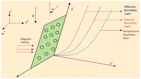
Consider time-dependent MHD in order to account stable mass diffusion within the presence having a heat source & energy dissipation associated with viscosity with varying temperatures, a viscous, electrically conducting, incompressible flow interacts with an inclined plate. Perpendicular to the fluid flow applies a constant magnetic field, B, with an intensity of B0. When its y' is taken above the surface on an upward direction, the y'-axis is perpendicular at y' and orthogonal to the x'y'-plane. Figure 1 shows the problem's physical model.
Figure 1. Mathematical model of the problem
The fluid concentration and plate and fluid temperature are initially in that time t'≤0. The plate then initiates to vibrate within the particular plane on frequency ω' time t'>0, raising the plate's temperature along with fluid concentration, respectively. Thus, heat transfer over the x'- direction is thought to be insignificant in comparison to that in the y' direction. With the exception of pressure, all physical parameters are dependent on y' and t'. The generalized Ohm's law on taking Hall current into account is given by the study [19]:
$\overset{\to }{\mathop{J}}\,+\frac{{{\omega }_{\text{e}}}{{\tau }_{e}}}{{{B}_{0}}}\text{ }\left( \overset{\to }{\mathop{J}}\,\times \overset{\to }{\mathop{B}}\, \right)=\sigma \left( \overset{\to }{\mathop{B}}\,+\overset{\to }{\mathop{q}}\,\times \overset{\to }{\mathop{B}}\, \right)$ (1)
where, $\vec{B}, \vec{q}, \vec{E}, \vec{J}, \sigma, \omega_e$ and $\tau_e$ are respectively, magnetic field vector, velocity vector, electric field vector, current density vector, electric conductively, cyclotron frequency and electron collision time.
The equation of continuity $\nabla \cdot \vec{q}=0$ gives v′=0 everywhere in the flow since there is no variation of the flow in y'- direction, where, $\vec{q}=\left(u^{\prime}, \mathrm{v}^{\prime} \,\,\mathrm{w}^{\prime}\right)$ and u′, v′, w′ are respectively, velocity components along the coordinate axes.
The magnetic Reynolds number is so small that the induced magnetic field produced by the fluid motion is neglected. The solenoid relation $\nabla \cdot \vec{B}=0$ for the magnetic field $\vec{B}=\left(B_{x^{\prime}}, B_y, B_{z^{\prime}}\right)$ gives $B_{y^{\prime}}=$ constant say $B_0$. i.e., $\vec{B}=\left(0, \,\,\mathrm{~B}_0, 0\right)$ everywhere in the flow. The conservation of electric current $\nabla \cdot \vec{J}=0$ yields $j_{y^{\prime}}=$ constant, where $\vec{J}=\left(j_{x^{\prime}}, \mathbf{J}_{y^{\prime}}, \mathbf{J}_{z^{\prime}}\right)$. This constant is zero since $j_{y^{\prime}}=0$ at the plate which is electrically non-conducting. Hence, $j_{y^{\prime}}=0$ everywhere in the flow. In view of the above assumption, Eq. (1) yields:
${{\text{J}}_{{{\text{x}}^{\text{ }\!\!'\!\!\text{ }}}}}\text{- m }{{\text{J}}_{{{\text{y}}^{\text{ }\!\!'\!\!\text{ }}}}}=\sigma \left( {{\text{E}}_{{{\text{x}}^{\text{ }\!\!'\!\!\text{ }}}}}-{w}'{{\text{B}}_{\text{0}}} \right)$ (2)
$\mathrm{xJ}_{\mathrm{Z}^{{\prime}^{\prime}}}-\mathrm{mJ}_{\mathrm{x}^{{\prime}^{\prime}}}=\sigma\left(\mathrm{E}_{\mathrm{Z}^{\prime}}+u^{\prime} \mathrm{B}_0\right)$ (3)
where, $m\left(=\omega_e \tau_e\right)$ is the Hall parameter which represents the ratio of electron-cyclotron frequency and the electron-atom collision frequency. Since the induced magnetic field is neglected, Maxwell equation $\nabla \times \vec{E}=\frac{\partial \vec{H}}{\partial t}$ becomes $\nabla \times \vec{E}=$ 0 which gives $\frac{\partial E_{x^{\prime}}}{\partial y^{\prime}}=0$ and $\frac{\partial E_{Z^{\prime}}}{\partial y^{\prime}}=0$. This implies that $\mathrm{E}_{\mathrm{x}^{\prime}}=$ constant everywhere in the flow and choose this constant equal to zero, i.e. $E_{x^{\prime}}=E_{Z^{\prime}}=0$ solving for $J_{x^{\prime \prime}}$ and $J_{Z^{\prime \prime}}$ from Eqs. (2) and (3) on using $E_{x^{\prime}}=\mathrm{E}_{Z^{\prime}}=0$.
$J_{X^{\prime}}=\frac{\sigma B_0}{\left(1+m^2\right)}\left(m u^{\prime}-w^{\prime}\right)$ (4)
$J_{z^{\prime}}=\frac{\sigma B_0}{\left(1+m^2\right)}\left(m w^{\prime}+u^{\prime}\right)$ (5)
Taking into consideration the assumptions made above, under the Boussinesq’s approximation, and using Eqs. (4) and (5), the basic governing equations of the flow are derived as.
The description of the physical problem closely follows that of Kumari et al. [18]. This introduces unsteadiness in the flow field. The physical model and the coordinate system are shown Figure 1.
Continuity equation:
$\frac{\partial v *}{\partial y^{\prime}}=0$ (6)
Momentum equation:
$\begin{array}{r}\frac{\partial u *}{\partial t^{\prime}}=v \frac{\partial^2 u *}{\partial y^{\prime 2}}+g \beta\left(T^{\prime}-T_{\infty}^{\prime}\right) \cos \alpha+g \beta^{\prime}\left(C^{\prime}-C_{\infty}^{\prime}\right) \cos \alpha -\frac{\sigma B_0^2}{\rho\left(1+m^2\right)}(u *+m w *)-\frac{v}{K_1} u *\end{array}$ (7)
$\frac{\partial w^*}{\partial t^{\prime}}=v \frac{\partial^2 w *}{\partial y^{\prime 2}}+\frac{\sigma B_0^2}{\rho\left(1+m^2\right)}(m u *-w *)-\frac{v}{K_1} w *$ (8)
Energy equation:
$\begin{aligned} & \rho C_P \frac{\partial T^{\prime}}{\partial t^{\prime}}=k \frac{\partial^2 T^{\prime}}{\partial y^{\prime 2}}-\frac{\partial q_r^{\prime}}{\partial y^{\prime}}+\mu\left(\frac{\partial u *}{\partial y^{\prime}}\right)^2-Q_0\left(T^{\prime}-T_{\infty}^{\prime}\right) +Q_l\left(C^{\prime}-C_{\infty}^{\prime}\right)+\left(\frac{D_m k_T \rho}{C_S}\right) \frac{\partial^2 C^{\prime}}{\partial y^{\prime 2}}\end{aligned}$ (9)
Concentration equation:
$\frac{\partial C^{\prime}}{\partial t^{\prime}}=D \frac{\partial^2 C^{\prime}}{\partial y^{\prime 2}}-K_c\left(C^{\prime}-C_{\infty}^{\prime}\right)+D_1 \frac{\partial^2 T^{\prime}}{\partial y^{\prime 2}}$ (10)
They specified initial and boundary conditions are:
$\begin{gathered}t^{\prime} \leq 0 ; u *=0, w *=0, T^{\prime}=T_{\infty}^{\prime}, C^{\prime}=C_{\infty}^{\prime} \text { for all } y^{\prime} \geq 0 t^{\prime}>0 ; \\ u *=u_0 \cos \omega^{\prime} t^{\prime}, w *=0\,\,\,\, T^{\prime}=T_{\infty}^{\prime}+\left(T_w^{\prime}-T_{\infty}^{\prime}\right) \frac{t u_0^2}{v}, C^{\prime} =C_w^{\prime} \text { as } y^{\prime}=0\end{gathered}$ (11)
$u * \rightarrow 0, w * \rightarrow 0, T^{\prime} \rightarrow T_{\infty}^{\prime}, C^{\prime} \rightarrow C_{\infty}^{\prime}$ as $y^{\prime} \rightarrow \infty$
Radiation energy flux ($q_r$) as stated by Roseland approximation:
${{q}_{r}}=\frac{4{{\sigma }^{\prime }}}{3{{k}^{\prime }}}\frac{\partial {{T}^{\prime 4}}}{\partial {{y}^{\prime }}}$ (12)
where, $\sigma^{\prime}$ is the Stefan-Boltzmann constant and $k^{\prime}$ is the mean absorption coefficient. It is assumed that temperature difference within the flow are sufficiently small, then Eq. (11) can be liberalized by expanding $T^{\prime 4}$ into the Taylor series about $T_{\infty}^{\prime}$ which, after neglecting higher-order terms, takes the form:
$T^{\prime 4} \cong 4 T_{\infty}^{\prime 3} T^{\prime}-3 T_{\infty}^{\prime 4}$ (13)
With reference to Eqs. (11) and (12), then Eq. (9) goes to:
$\begin{gathered}\rho C_P \frac{\partial T^{\prime}}{\partial t^{\prime}}=k\left(1+\frac{16 \sigma^{\prime} T_{\infty}^{\prime 3}}{3 k k^{\prime}}\right) \frac{\partial^2 T^{\prime}}{\partial y^{\prime 2}}+\mu\left(\frac{\partial u^{\prime}}{\partial y^{\prime}}\right)^2-Q_0\left(T^{\prime}-T_{\infty}^{\prime}\right) +Q_l\left(C^{\prime}-C_{\infty}^{\prime}\right)+\left(\frac{D_m k_T \rho}{C_S}\right) \frac{\partial^2 C^{\prime}}{\partial y^{\prime 2}}\end{gathered}$ (14)
On introducing the following non-dimensional quantities,
$\begin{gathered}u=\frac{u *}{u_0}, w=\frac{w *}{u_0} y=\frac{u_0 y^{\prime}}{v}, t=\frac{t^{\prime} u_0^2}{v}, \omega=\frac{\omega^{\prime} v}{u_0^2} \theta=\frac{T^{\prime}-T_{\infty}^{\prime}}{T_w^{\prime}-T_{\infty}^{\prime}}, C=\frac{C^{\prime}-C_{\infty}^{\prime}}{C_w^{\prime}-C_{\infty}^{\prime}} \\ \operatorname{Pr}=\frac{\mu C_p}{k}, S c=\frac{v}{D}, M=\frac{\sigma \mu_0^2 H_0^2 v}{\rho v_0^2}, G r=\frac{v g \beta\left(T_w^{\prime}-T_{\infty}^{\prime}\right)}{u_0^3}, G m=\frac{v g \beta^{\prime}\left(C_w^{\prime}-C_{\infty}^{\prime}\right)}{u_0^3} \\ K=\frac{K_1 u_0^2}{v^2}, K r=\frac{v K_c}{u_0^2}, R=\frac{16 \sigma^{\prime} T_{\infty}^3}{3 k \kappa^{\prime}}, Q=\frac{Q_0}{\rho C_P v}, R_a=\frac{Q_l v\left(C_w^{\prime}-C_{\infty}^{\prime}\right)}{\rho C_P u_0^2\left(T_w^{\prime}-T_{\infty}^{\prime}\right)}\end{gathered}$ (15)
$E_C=\frac{u_0^2}{C_P\left(T_w^{\prime}-T_{\infty}^{\prime}\right)} D f=\frac{D_m k_T\left(C_w^{\prime}-C_{\infty}^{\prime}\right)}{v C_S C_P\left(T_w^{\prime}-T_{\infty}^{\prime}\right)}$ from above measures (15), Eqs. (7), (8), (14) and (10) reduce in the form:
$\begin{gathered}\frac{\partial u}{\partial t}=\frac{\partial^2 u}{\partial y^2}-\left(\frac{M}{1+m^2}\right)(u+m w)+G r \cos \alpha \theta +G m \cos \alpha C-\frac{u}{K}\end{gathered}$ (16)
$\frac{\partial w}{\partial t}=\frac{{{\partial }^{2}}w}{\partial {{y}^{2}}}+\left( \frac{M}{1+{{m}^{2}}} \right)(mu-w)-\frac{w}{K}\,$ (17)
$\frac{\partial \theta}{\partial t}=\left(\frac{1+R}{P r} O \frac{\partial^2 \theta}{\partial y^2}{ }_a \frac{\partial^2 C}{\partial y^2}{ }_C\left(\frac{\partial u}{\partial y}\right)^2\right)$ (18)
$\frac{\partial C}{\partial t}=\frac{1}{S c} \frac{\partial^2 C}{\partial y^2}-K r C+S_0 \frac{\partial^2 \theta}{\partial y^2}$ (19)
Eq. (11) with initial also edge circumstances through non-dimensional have becomes:
$\begin{aligned} & t \leq 0 ; u=0, w=0, \theta=0 C=0 \text { forally } \geq 0 \\ & t>0 ; u=\operatorname{Cos} \omega t, w=0, \theta=t, C=1 \text { aty }=0 \\ & u \rightarrow 0 w \rightarrow 0 \theta \rightarrow 0 C \rightarrow 0 \text { asy } \rightarrow \infty\end{aligned}$ (20)
Eqs. (16)-(19) are linear partial differential equations and are to be solved by using the initial and boundary conditions (20). However exact solution is not possible for this set of equations and hence we solve these equations by finite-difference method. The equivalent finite difference schemes of equations for (16)-(19) are as follows:
$\begin{aligned} \frac{u_{i^*, j^*+1}-u_{i^*, j^*}}{\Delta t}= & \frac{u_{i^*-1, j^*}-2 u_{i^*, j^*}+u_{i^*+1, j^*}}{(\Delta y)^2} -\left(\frac{M}{1+m^2}\right)\left(u_{i^*, j^*}+m w_{i^*, j^*}\right)+G r \cos \alpha \theta_{i^*, j^*} +G m \cos \alpha C_{i^*, j^*}-\frac{u_{i^*, j^*}}{K}\end{aligned}$ (21)
$\frac{w_{i^*, j^*+1}-w_{i^*, j^*}}{\Delta t}=\frac{w_{i^*-1, j^*}-2 w_{i^*, j^*}+w_{i^*+1, j^*}}{(\Delta y)^2}+\left(\frac{M}{1+m^2}\right)\left(m u_{i^*, j^*}-w_{i^*, j^*}\right)-\frac{w_{i^*, j^*}}{K}$ (22)
$\begin{aligned} & \frac{\theta_{i^*, j^*+1}-\theta_{i^*, j^*}}{\Delta t} \\ & =\left(\frac{1+R}{\operatorname{Pr}}()\left(\frac{\theta_{i^*-1, j^*}-2 \theta_{i^*, j^*}+\theta_{i^*+1, j^*}}{(\Delta y)^2}\right)_{i^*, j^* a_{i^*, j^*}}\right) \\ & +D u\left(\frac{C_{i^*-1, j^*}-2 C_{i^*, j^*}+C_{i^*+1, j^*}}{(\Delta y)^2}\right)+E_C\left(\frac{u_{i^*, j^*+1}-u_{i^*, j^*}}{\Delta t}\right)^2\end{aligned}$ (23)
$\frac{C_{i^*, j^*+1}-C_{i^*, j^*}}{\Delta t}=\left(\frac{1}{S c}\right)\left(\frac{C_{i^*-1, j^*}-2 C_{i^*, j^*}+C_{i^*+1, j^*}}{(\Delta y)^2}\right)-K r C_{i^*, j^*}+S_0\left(\frac{\theta_{i^*-1, j^*}-2 \theta_{i^*, j^*}+\theta_{i^*+1, j^*}}{(\Delta y)^2}\right)$ (24)
Here, the suffixes i* & j* stand for y and time (t) respectively. To split the mesh system, take ∆y = 0.05. The equivalent of the starting condition in (20) is as follows:
$u\left(i^*, 0\right)=0, w\left(i^*, 0\right)=0, \theta\left(i^*, 0\right)=0, C\left(i^*, 0\right)=0$ for all $i$ (25)
The following is a finite-difference form of the boundary constraints given (20).
$u\left(i^*, 0\right)=\operatorname{Cos} \omega t, w\left(i^*, 0\right)=0, \theta\left(i^*, 0\right)=t, C\left(i^*, 0\right)=1 a t y=0$
$u\left(i^* *^* *^* *^* *^* {{\max}_{{{\max}_{{\max}_{\max}}}}}\right)$ (26)
(Here $i_{\max }^*$ was taken as 200).
In regard to temperature, concentration, or velocity at sites on the prior time-step, the final velocity for each time step, your (“i*, j*+1) (i*=1,200) & w (i*, j*+1) (i* = 1”,200), are first computed using (21) & (22). Then, using Eqs. (23) and (24), we compute θ (i*, j*+1) along with C (i*, j*+1), respectively. This procedure keeps going until j* = 5000, or t = 0.5. 0.0001 was chosen as ∆t for the calculation.
Skin-friction:
The dimensionless expressions for main and minor skin friction are expressed as follows:
$\tau_x=\frac{\partial u}{\partial y}$ aty $=0$ and $\tau_z=\frac{\partial w}{\partial y}$ aty $=0$
Rate of heat transfer:
The non- dimension proportion of temperature transmission is specified through:
$N u=\frac{\partial \theta}{\partial y} a t y=0$
Rate of mass transfer:
The non-dimensional expression for the rate of mass transmission is represented as:
$S h=\frac{\partial C}{\partial y}$ aty $=0$
Result and discussion:
The parameters like Grashof number (Gr = 10), the modified Grashof number (Gm = 10), magnetic parameter (M = 2), Hall current (m = 0.5), Dufour parameter (Df = 0.5), Permeability parameter (K = 0.5), Prandtl number (Pr = 0.71), Heat Source (Q = 2), Radiation Parameter (R = 2), Oscillation frequency ($\omega=\pi / 6$, Soret parameter (S0 = 2), Eckert number (E0.1), Schmidt number (Sc = 0.22) and Chemical reaction parameter (Kr = 0.5).
From the Figures 2 to 7 shows that primary and secondary fluid velocities in cooled and heated plates and Figures 8 to 11 show the effects of different parameters such as “R, Q, Ra and Du” on temperature distribution and also observed the behavior of the Figures 12 to 13 on concentration profiles respectively.
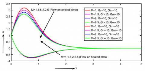
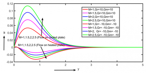
Figures 2 and 3 show that as the magnetic field parameter is increased, the primary and secondary velocity fields through cooled plates decrease, and the opposite effect occurs in heated plates. The reason for this is that the introduction of a transverse magnetic field will produce a Lorentz force, which is a resistive force that acts like a drag force and seeks to impede fluid flow, hence decreasing fluid velocity.
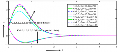
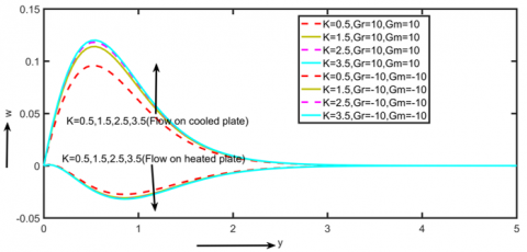
It is evident from Figures 4 and 5 that increasing K values cause a rise in primary and secondary velocities. In terms of physics, an increase in K tends to reduce the porous medium's resistance, which increases the fluid's velocity across cooled plates and has the reverse effect on heated plates.
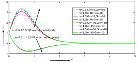
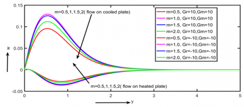
The impact of Hall current on primary and secondary velocities (u, w), as depicted in Figures 6 and 7. It is clear from Figures 5 and 6 that the primary velocity "u" grows at increasing "m" around the boundary layer field, while the secondary velocity w decreases with increasing "m" throughout the boundary layer area on the cooled plate and also has the opposite effect on the heated plate. Given that Hall current creates secondary flow in the flow-field and has the opposite effect on primary fluid velocity throughout the boundary layer region, it follows that Hall current tends to accelerate primary fluid velocity throughout the boundary layer region.
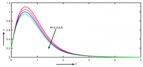
Radiation parameter "R" values, as seen in Figure 8, raise temperature profiles, but greater radiation parameter values just increase surface heat transfer, which raises the fluid's temperature.
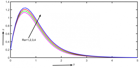
The effect of temperature "Ra" is seen in Figure 9. When radiation absorption increases, the thermal boundary layer rises. Physically, the large "Ra" values correspond to an increased radiation by conduction over absorption, which causes the buoyant force and thickness of the thermal boundary layers to rise.
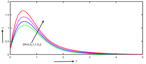
The impact of the Dufour number "Df" on temperature profiles is shown in Figures 10. Heat flux generated by a concentration gradient is referred to as the Dufour effect. Compared to when the Dufour effect is absent, the temperature profiles are greater when the Dufour effect is present. As a result, the boundary layer flow becomes more energetic as the Dufour number rises, and the thermal boundary layer thickness significantly rises when Dufour effects are present.
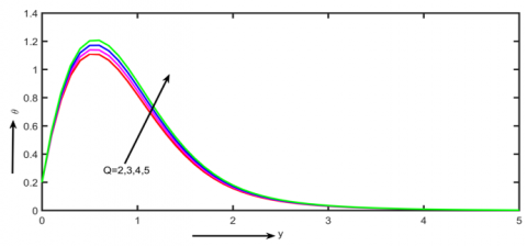
Figure 11 displays the temperature profiles for various values of the heat source parameter "Q." With rising levels of "Q," it is noted that the temperature field is decaying. The numerical findings demonstrate that the heat source effects have a propensity to lower the fluid temperature and that larger values of "Q" have the impact of decreasing the thermal boundary layer thickness and enhancing uniformity across the boundary layer in temperature distribution.
Figure 2. Effect of magnetic parameter on primary velocity
Figure 3. Effect of magnetic parameter on secondary velocity
Figure 4. Effect of porosity parameter on primary velocity
Figure 5. Effect of porosity parameter on secondary velocity
Figure 6. Effect of hall parameter on primary velocity
Figure 7. Effect of hall parameter on secondary velocity
Figure 8. Effect of radiation parameter on temperature
Figure 9. Effect of radiation absorption parameter on temperature
Figure 10. Effect of Dufour parameter on temperature
Figure 11. Effect of heat source parameter on temperature
Figure 12. Effect of Schmidt number on concentration
Figure 13. Effect of chemical reaction parameter on concentration
Figure 12 shows how the Schmidt number (Sc) behaves on the concentration curves. The mass diffusivity to momentum ratio is represented by the Schmidt number Sc. It measures the relative efficiency of mass transfer and momentum in the hydrodynamic (velocity) & concentration (species) boundary layer through diffusion. Greater Schmidt numbers cause the fluid's mass diffusivity to decrease, which lowers the concentration profiles.
The impact on the concentration profiles of the chemical reaction factor is seen in Figure 13. This review examines the effects of a harmful chemical reaction (Kr>0). The concentration distributions decrease with increasing chemical reaction. A chemical reaction occurs physically with several conflicts leading to a devastating situation. In essence, this lowers the fluid flow concentration distribution by increasing transport and inducing high molecular mobility.
RSM serves as an effective approach for analysing multiple variables using limited resources, measurable data, and structured experimental design. The main phases in RSM can be outlined as shadows.
1). The data values are systematically planned and analysed to obtain reliable and valid estimates aimed at the predicted answer
2). The greatest appropriate accurate representations were pronounced for the answer exterior
3). It stood established that response surface accurate replicas provide the most appropriate representation
4). ANOVA was accomplished to examine both the direct and interaction possessions of the parameters
5.1 Optimization analysis by RSM
The association concerning the answer adjustable with the influencing factors was evaluated expending a face-cantered central composite design. Table 1 demonstrations the ranges and stages of the key constraints, incorporating linear, quadratic, and interaction terms.
Table 1. Constraints with their levels for $S_h, T_x$ and $N u$
|
Parameter |
Representation |
Level |
Low (-1) |
Middle (0) |
High (+1) |
|
$0.22 \leq S_c \leq 2$ |
S1 |
$S_h$ |
0.22 |
0.725 |
2 |
|
$0.5 \leq S_0 \leq 2$ |
S2 |
0.5 |
1.25 |
2 |
|
|
$10 \leq K_r \leq 40$ |
S3 |
10 |
25 |
40 |
|
|
$1 \leq M \leq 2.5$ |
S1 |
$T_x$ |
1 |
1.75 |
2.5 |
|
$5 \leq G_m \leq 15$ |
S2 |
5 |
10 |
15 |
|
|
$1 \leq D_u \leq 3$ |
S3 |
1 |
4 |
3 |
|
|
$1 \leq R \leq 30$ |
S1 |
Nu |
1 |
15.5 |
30 |
|
$\begin{aligned} & 0.71 \leq P_r \leq 2.36\end{aligned}$ |
S2 |
0.71 |
1.535 |
2.36 |
|
|
$1 \leq R_a \leq 30$ |
S3 |
1 |
15.5 |
30 |
$\begin{aligned} \text { Response }=a_0 & +a_1 S_1+a_2 S_2+a_3 S_3+a_{11} S_1{ }^2+a_{22} S_2{ }^2 \\ & +a_{33} S_3{ }^2+a_{12} S_1 S_2+a_{13} S_1 S_3+a_{23} S_2 S_3\end{aligned}$
5.1.1 Response surface regression: $\tau$
RSM is employed as a robust statistical approach to explain the relationships concerning important constraints—such as Sc, So, and Kr; M, Gm, and Du; and R, Pr, and Ra—and the response variables, namely, and Nu. The optimal configuration is identified, and a sensitivity analysis of the dominant factors influencing is conducted. Table 2 presents the response function values obtained from 20 investigational innings. The multivariate perfect representing the replies as purposes of the important constraints is expressed as surveys.
Table 2. Investigational proposal with replies for $S_h, T_x$ and Nu
|
Actual Values |
Retorts |
Actual Values |
Retorts |
Actual Values |
Retorts |
|||||||
|
S. No |
Sc |
So |
Kr |
Sh |
M |
Gm |
Du |
Tx |
R |
Pr |
Ra |
Nu |
|
1 |
2 |
2 |
40 |
2.5735 |
2.5 |
15 |
3 |
1.6455 |
30 |
2.36 |
30 |
-3.6336 |
|
2 |
0.735 |
1.25 |
25 |
6.4413 |
1.75 |
10 |
2 |
1.7761 |
15.5 |
1.535 |
15.5 |
-1.4128 |
|
3 |
2 |
1.25 |
25 |
12.481 |
2.5 |
10 |
2 |
1.776 |
30 |
1.535 |
15.5 |
-1.5044 |
|
4 |
0.735 |
2 |
25 |
1.142 |
1.75 |
15 |
2 |
1.7772 |
15.5 |
2.36 |
15.5 |
-3.8683 |
|
5 |
0.22 |
1.25 |
25 |
4.1485 |
1 |
10 |
2 |
1.7761 |
1 |
1.535 |
15.5 |
-1.3198 |
|
6 |
0.735 |
1.25 |
10 |
6.0458 |
1.75 |
10 |
1 |
2.1367 |
15.5 |
1.535 |
1 |
-1.6742 |
|
7 |
2 |
2 |
10 |
1.1238 |
2.5 |
15 |
1 |
2.1377 |
30 |
2.36 |
1 |
-4.2528 |
|
8 |
0.735 |
1.25 |
40 |
6.8306 |
1.75 |
10 |
3 |
1.6443 |
15.5 |
1.535 |
30 |
-1.1529 |
|
9 |
0.22 |
0.5 |
40 |
5.6395 |
1 |
5 |
3 |
1.6432 |
1 |
0.71 |
30 |
2.6541 |
|
10 |
2 |
0.5 |
40 |
19.828 |
2.5 |
5 |
3 |
1.6431 |
30 |
0.71 |
30 |
2.4511 |
|
11 |
0.735 |
1.25 |
25 |
6.4413 |
1.75 |
10 |
2 |
1.7761 |
15.5 |
1.535 |
15.5 |
-1.4128 |
|
12 |
0.22 |
0.5 |
10 |
5.2791 |
1 |
5 |
1 |
2.1358 |
1 |
0.71 |
1 |
2.3306 |
|
13 |
2 |
0.5 |
10 |
19.2049 |
2.5 |
5 |
1 |
2.1357 |
30 |
0.71 |
1 |
2.1316 |
|
14 |
0.735 |
1.25 |
25 |
6.4413 |
1.75 |
10 |
2 |
1.7761 |
15.5 |
1.535 |
15.5 |
-1.4128 |
|
15 |
0.735 |
0.5 |
25 |
10.3171 |
1.75 |
5 |
2 |
1.775 |
15.5 |
0.71 |
15.5 |
2.3916 |
|
16 |
0.735 |
1.25 |
25 |
6.4413 |
1.75 |
10 |
2 |
1.7761 |
15.5 |
1.535 |
15.5 |
-1.4128 |
|
17 |
0.22 |
2 |
40 |
2.8932 |
1 |
15 |
3 |
1.6456 |
1 |
2.36 |
30 |
-3.4791 |
|
18 |
0.735 |
1.25 |
25 |
6.4413 |
1.75 |
10 |
2 |
1.7761 |
15.5 |
1.535 |
15.5 |
-1.4128 |
|
19 |
0.735 |
1.25 |
25 |
6.4413 |
1.75 |
10 |
2 |
1.7761 |
15.5 |
1.535 |
15.5 |
-1.4128 |
|
20 |
0.22 |
2 |
10 |
2.458 |
1 |
15 |
1 |
2.1378 |
1 |
2.36 |
1 |
-4.1092 |
Table 3. Coded coefficients
|
Term |
Coefficient |
Standard Error |
T-Value |
P-Value |
VIF |
|
Constant |
8.001 |
0.167 |
47.81 |
0 |
|
|
Sc |
3.517 |
0.155 |
22.73 |
0 |
1.03 |
|
So |
-5.314 |
0.16 |
-33.28 |
0 |
1.01 |
|
Kr |
0.365 |
0.159 |
2.3 |
0.038 |
1 |
|
So*So |
-0.659 |
0.228 |
-2.88 |
0.012 |
1.03 |
|
Sc*So |
-3.636 |
0.175 |
-20.81 |
0 |
1.01 |
Table 4. Analysis of variance (ANOVA) for Sh
|
Source |
Degrees of Freedom (DF) |
Sequential Sums of Squares |
Contribution |
Adj Sum of Squares |
Adjusted Mean Squares |
F-Value |
P-Value |
|
Model |
5 |
492.616 |
99.29% |
492.616 |
98.523 |
389.59 |
0 |
|
Linear |
3 |
380.981 |
76.79% |
412.048 |
137.35 |
543.13 |
0 |
|
Sc |
1 |
128.865 |
25.97% |
130.704 |
130.7 |
516.85 |
0 |
|
So |
1 |
250.782 |
50.54% |
280.01 |
280.01 |
1107.3 |
0 |
|
Kr |
1 |
1.335 |
0.27% |
1.335 |
1.335 |
5.28 |
0.038 |
|
Square |
1 |
2.105 |
0.42% |
2.105 |
2.105 |
8.32 |
0.012 |
|
So*So |
1 |
2.105 |
0.42% |
2.105 |
2.105 |
8.32 |
0.012 |
|
2-Way Interaction |
1 |
109.53 |
22.08% |
109.53 |
109.53 |
433.12 |
0 |
|
Sc*So |
1 |
109.53 |
22.08% |
109.53 |
109.53 |
433.12 |
0 |
|
Error |
14 |
3.54 |
0.71% |
3.54 |
0.253 |
||
|
Lack-of-Fit |
9 |
3.54 |
0.71% |
3.54 |
0.393 |
* |
* |
|
Pure Error |
5 |
0 |
0.00% |
0 |
0 |
||
|
Total |
19 |
496.156 |
100.00% |
Table 5. Coded coefficients
|
Term |
Coeff |
SE Coeff |
T-Value |
P-Value |
VIF |
|
Constant |
-1.41281 |
0.00278 |
-508.66 |
0 |
|
|
R |
-0.08847 |
0.00278 |
-31.85 |
0 |
1 |
|
Pr |
-3.1302 |
0.00278 |
-1126.98 |
0 |
1 |
|
Ra |
0.24136 |
0.00278 |
86.9 |
0 |
1 |
|
Pr*Pr |
0.67441 |
0.00393 |
171.69 |
0 |
1 |
|
R*Pr |
0.01299 |
0.00311 |
4.18 |
0.001 |
1 |
|
Pr*Ra |
0.07579 |
0.00311 |
24.41 |
0 |
1 |
Table 6. Analysis of variance (ANOVA) for Tx
|
Source |
DF |
Seq SS |
Contribution |
Adj SS |
Adj MS |
F-Value |
P-Value |
|
Model |
6 |
100.964 |
100.00% |
100.964 |
16.8273 |
218122 |
0 |
|
Linear |
3 |
98.642 |
97.70% |
98.642 |
32.8808 |
426213.5 |
0 |
|
R |
1 |
0.078 |
0.08% |
0.078 |
0.0783 |
1014.56 |
0 |
|
Pr |
1 |
97.982 |
97.05% |
97.982 |
97.9815 |
1270075 |
0 |
|
Ra |
1 |
0.583 |
0.58% |
0.583 |
0.5825 |
7551.19 |
0 |
|
Square |
1 |
2.274 |
2.25% |
2.274 |
2.2741 |
29478.34 |
0 |
|
Pr*Pr |
1 |
2.274 |
2.25% |
2.274 |
2.2741 |
29478.34 |
0 |
|
2-Way Interaction |
2 |
0.047 |
0.05% |
0.047 |
0.0236 |
306.56 |
0 |
|
R*Pr |
1 |
0.001 |
0.00% |
0.001 |
0.0013 |
17.49 |
0.001 |
|
Pr*Ra |
1 |
0.046 |
0.05% |
0.046 |
0.0459 |
595.62 |
0 |
|
Error |
13 |
0.001 |
0.00% |
0.001 |
0.0001 |
||
|
Lack-of-Fit |
8 |
0.001 |
0.00% |
0.001 |
0.0001 |
* |
* |
|
Pure Error |
5 |
0 |
0.00% |
0 |
0 |
||
|
Total |
19 |
100.965 |
100.00% |
i) Statistical Analysis
Under the quantified conditions, the statistical investigation was performed with 20 turns for Sh. Tables 3 and 4 present the coded coefficients and the effects of the statistical evaluation. The model demonstrates strong suitability for predicting Sh, with an R² value of 99.29% obtained through the applied statistical approach. Additionally, the adjusted R² for Sh is 99.03%. An R² of 98.21% designates that the perfect successfully explains nearly all the variation in the answer adjustable about its mean. In general, a higher R² reflects a better regression fit to the observed data.
ii) ANOVA and Model Estimation
To obtain the regression expression, the investigational perfect outlined in Table 4 was implemented below varying investigational conditions. The outstanding plot was generated through analysis of variance by processing the information with statistical package.
The validity of the regression representations is verified concluded ANOVA and diagnostic plots, supported by several statistical examinations presented in the equivalent tables. The effectiveness of the typical with the variation in the data are assessed using p-values and F-values. Terms with an F-value ≥1 and a p-value <0.05 are retained in the model, highlighting their importance in manufacturing applications, while irrelevant relations are excluded to improve model accuracy.
The standard probability figure exposes that entirely remainders support thoroughly through the traditional contour, representative standard standard circulation of mistakes. Furthermore, the bar chart for Sh guesstimates a bell shape, Normality is additional verified, which displays the residual plots for Sh, indicating that the residuals conform to a normal distribution. The residual histogram supports this finding by exhibiting a uniform spread. In addition, the largest residuals are highlighted, enabling closer examination and validation.
Although the main residuals were identified, the complete residual design confirms that the regression perfect is healthy and delivers a consistent fit. The residual comportment reflects the model’s effectiveness in capturing the inconsistency of the answer flexible Sh. This validates the suitability of the industrialized quadratic polynomial classical for the present study. Moreover, the residual plots show a random error distribution, fulfilling a key supposition for the credibility of regression representations.
These findings cooperatively specify that the selected prototypical is appropriate and delivers a strong fit. By eliminating inconsequential standings, the prototypical is advanced, thereby improving its analytical accuracy and steadfastness. The simplified deterioration typical intended for Sh, resulting from comprehensive arithmetical investigation and ANOVA results, is therefore obtainable. This advanced perfect, validated through demanding algebraic testing, effectively captures the essential associations concerning the important constraints and the answer variable quantity in this study.
iii) Regression Equation in Uncoded Units
The advanced model, validated through comprehensive statistical analysis, effectively captures the critical associations between the substantial restrictions and the response variables in this study.
$\begin{gathered}\mathrm{Sh}=2.475+10.761 \mathrm{Sc}+1.89 \mathrm{So}+0.0244 \mathrm{Kr} -1.171 \mathrm{So}^* \mathrm{So}-5.447 \mathrm{Sc}{ }^* \mathrm{So}\end{gathered}$
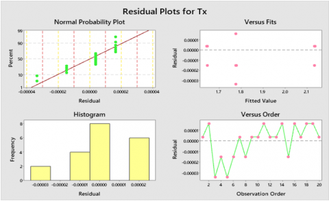
iv) Residual and Contour Plots
Figure 14 presents the residual plot, where the residuals represent the alterations concerning the observed and predicted y-values. The normal probability plot indicates good conformity to normality, as most points lie close to the approximate straight line. In the residual histogram, the splits are not perfectly symmetric, indicating a slightly skewed distribution. Comparison of experiential and tailored values shows good correlation, as reflected in the residuals versus fitted values diagram.
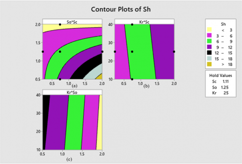
Figures 15 (a)-(c) display contour plots for Sh, providing a graphic symbolization of the properties of collaboration relations on Sh. These plots illustrate the combined influence of two key constraints on Sh. By imagining these connections, the contour plots offer insights into in what way parameter variations impact the response, aiding in understanding system behaviour and optimization.
v) Factorial plots for Sh
Figures 16 (a)-(c) depicts the interaction plots for Sh, illustrating how the consequence of one issue may depend on the smooth of additional. Such interactions are important for optimizing experimental or simulation conditions.
Figure 14. Residual vs. observation for Sh
Figure 15. For numerous constraint connections, contour plots (a) through (c) illustrate Sh
Figure 16. For numerous constraint connections, Interaction plots (a) through (c) illustrate Sh
Figure 17. (a) Consequence of Sc and So on Sh (b) Outcome of Sc and Kr on Sh (c) Influence of So and kr on Sh
Figure 18. Error vs. observation for Tx
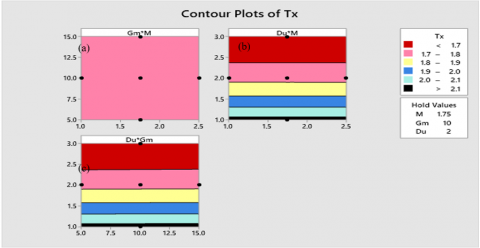
Figure 19. For numerous constraint connections, contour plots (a) through (c) illustrate Tx
vi) Surface Plots
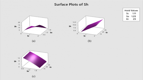
Figures 17 depicts the surface plots for Sh.
5.1.2 Response surface regression: Tx
This section investigates the effect of three factors $\mathrm{M}, G_m$ and $D_u$ on Tx. The optimal configuration is identified, and a sensitivity analysis of the influential factors on Tx is conducted.
i) Statistical Analysis
Under the quantified conditions, statistical investigation was carried out with 20 runs for Tx. Tables 5 and 6 present the coded coefficients and the effects of the statistical evaluation. The model is suitable for predicting Tx, as it achieved an R² value of 100% through the applied statistical approach. Additionally, the adjusted R² for Tx is 100%, slightly lower than R², yet the model still provides an acceptable fit to the experimental data.
ii) Analysis of Variance and Model Estimation
To derive the estimated regression equation, the investigational classical in Table 6 was implemented under modified untried conditions. The outstanding plot was generated using analysis of variance and statistical software. Using RSM, the regression equation in uncoded units is obtained, representing the quantitative relationship among the significant factors.
iii) Regression Equation in Uncoded Units
$\begin{aligned} & \mathrm{Tx}=2.72465-0.000067 M+0.000155 \mathrm{Gm}-0.704125 \mathrm{Du} \\ & +0.000001 \mathrm{Gm}^* \mathrm{Gm}+0.114431 \mathrm{Du} * \mathrm{Du}+0.000020 \mathrm{Gm}^* \mathrm{Du}\end{aligned}$
iv) Residual and Contour Plots
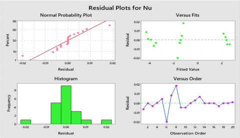
Figure 18 presents the residual plot, where residuals represent the differences between the observed and predicted y-values. The normal probability plot shows good conformity to normality, as most points lie close to the approximate straight line. In error histogram, the splits are not perfectly symmetric, indicating a slightly skewed distribution. Comparison of experiential and formfitting values demonstrates a strong association, as reflected in the residual versus formfitting values plot.
The contour plots for $\tau$ exposed in Figures 19, offer a diagram protest of the consequences of communication terms on Tx. These plots scrutinize the simultaneous communication linking two substantial boundaries on Tx. By imagining these connections, the contour plots help in sympathetic how variations in the constraints move the answer variables, contribution appreciated intuitions interested in the performance and optimization of the system.
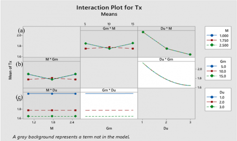
v) Factorial Plots for Tx
The Collaboration designs for Tx displayed in Figures 20 (a)-(c), current these interface designs can display whether interaction effects refer to the shared influence of two or more features on a response variable, which differs from the effect of each factor individually.
Figure 20. For numerous restriction connections, communication plots (a) through (c) illustrate Tx
Figure 21. (a) Consequence of Gm and M on Tx, (b) Consequence of M and Du on Tx, and (c) Impact of Gm and Du on Tx
vi) Surface Plots
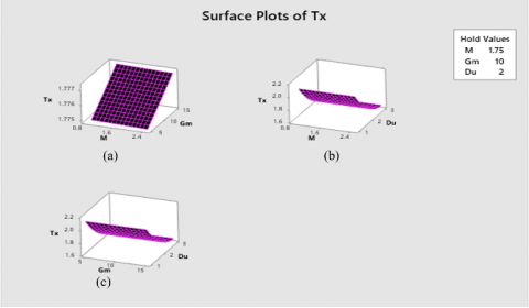
Figure 21(a) demonstrates the significance of Gm and M on retort purpose, the response function reached maximum value for the minimal value of Gm and M. Figures 21(b) and (c) explained the influence of M and Du on response function. The maximum value of the response function is experiential at small value of Gm and Du and all standards of Tx.
Response Surface Regression: Nu
This segment examines the effect of 3 issues R, $P_r$ in addition $R_a$ on Nu. The optimal configuration is determined, and a sensitivity analysis of the key factors influencing Nu is conducted.
i) Statistical Analysis
Under the specified conditions, statistical analysis was performed with 20 turns for Nu. Tables 7 with 8 present the oblique coefficients in addition the effects of the statistical evaluation. The model is appropriate for predicting Nu, achieving an R² value of 100% through the applied statistical method. Additionally, the adjusted R² for Nu is 100%, slightly lower than R², yet the model still provides an acceptable fit to the experimental data.
Table 7. Coded coefficients
|
Term |
Coeff |
SE Coeff |
T-Value |
P-Value |
VIF |
|
Constant |
-1.41281 |
0.00278 |
-508.66 |
0 |
|
|
R |
-0.08847 |
0.00278 |
-31.85 |
0 |
1 |
|
Pr |
-3.1302 |
0.00278 |
-1126.98 |
0 |
1 |
|
Ra |
0.24136 |
0.00278 |
86.9 |
0 |
1 |
|
Pr*Pr |
0.67441 |
0.00393 |
171.69 |
0 |
1 |
|
R*Pr |
0.01299 |
0.00311 |
4.18 |
0.001 |
1 |
|
Pr*Ra |
0.07579 |
0.00311 |
24.41 |
0 |
1 |
Table 8. Analysis of variance (ANOVA) for Nu
|
Source |
DF |
Seq SS |
Contribution |
Adj SS |
Adj MS |
F-Value |
P-Value |
|
Model |
6 |
100.964 |
100.00% |
100.964 |
16.8273 |
218122 |
0 |
|
Linear |
3 |
98.642 |
97.70% |
98.642 |
32.8808 |
426213.5 |
0 |
|
R |
1 |
0.078 |
0.08% |
0.078 |
0.0783 |
1014.56 |
0 |
|
Pr |
1 |
97.982 |
97.05% |
97.982 |
97.9815 |
1270075 |
0 |
|
Ra |
1 |
0.583 |
0.58% |
0.583 |
0.5825 |
7551.19 |
0 |
|
Square |
1 |
2.274 |
2.25% |
2.274 |
2.2741 |
29478.34 |
0 |
|
Pr*Pr |
1 |
2.274 |
2.25% |
2.274 |
2.2741 |
29478.34 |
0 |
|
2-Way Interaction |
2 |
0.047 |
0.05% |
0.047 |
0.0236 |
306.56 |
0 |
|
R*Pr |
1 |
0.001 |
0.00% |
0.001 |
0.0013 |
17.49 |
0.001 |
|
Pr*Ra |
1 |
0.046 |
0.05% |
0.046 |
0.0459 |
595.62 |
0 |
|
Error |
13 |
0.001 |
0.00% |
0.001 |
0.0001 |
||
|
Lack-of-Fit |
8 |
0.001 |
0.00% |
0.001 |
0.0001 |
* |
* |
|
Pure Error |
5 |
0 |
0.00% |
0 |
0 |
||
|
Total |
19 |
100.965 |
100.00% |
Figure 22. Error vs. observation for Nu
Figure 23. For several constraint interfaces, contour plots (a) through (c) illustrate Tx
Figure 24. For numerous constraint connections, Interaction plots (a) through (c) illustrate Nu
Figure 25. (a) Significance of Pr and R on Nu (b) Effect of Ra and R on Nu (c) Impact of Pr and Ra on Nu
iii) Model Representation Using Real Variables
Nu=6.7591-0.007768 R-6.9512 Pr+0.006921 Ra+0.99087 Pr*Pr+0.001086 R*Pr+0.006335 Pr*Ra
iv) Residual and Contour Plots
The Error plot is presented in Figure 22. In this plot, the Error represents the alteration between the experiential values from the scatter diagram and the projected y-values. The normal probability plot appears satisfactory, as most data points lie close to a straight line, indicating normality. However, the residual histogram is not perfectly symmetric, suggesting a skewed distribution. A comparison of the residual diagram with the fitted values shows that the observed and predicted values exhibit a strong correlation.
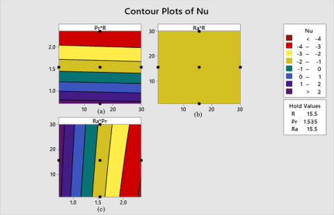
Figures 23 (a-c) present the contour plots for Nu, which illustrate the interactive effects of paired parameters on the response. These plots highlight the combined influence of two key variables on Nu. By depicting these connections, the contour plots provide a clearer considerate of in what way variations in the restrictions influence the answer variable, thereby contribution useful intuitions into system behaviour and optimization.
v) Factorial Plots for Nu
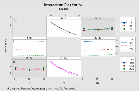
The Interface plots for Nu exposed in Figures 24 (a)-(c), existing these contact diagrams can demonstrate if interaction effects refer to the mutual influence of two or more influences on a response variable, which differs from the effect of each factor individually.
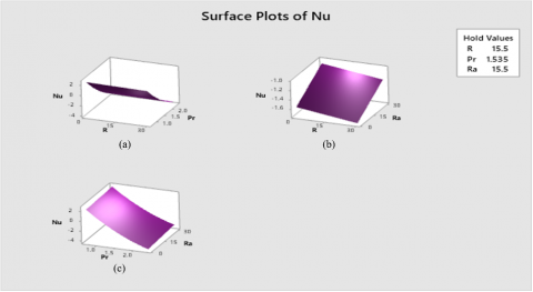
vi) Surface Plots
Figure 25(a) demonstrates the significance of Pr and R on response function. It achieved supreme value for the nominal value Pr and R Figures 25(b), (c) explained the influence of of Ra and R on answer function. The maximum value of the response function is experiential at short value of Pr and Ra and all values of Nu.
This work investigates the numerical analysis of Hall current and viscous dissipation properties on instable MHD free convective movement previous and disposed permeable shield, employing both the FDM and RSM. The model incorporates the stimuluses of Hall current, Dufour outcome, viscid indulgence, and a thermal basis. The dimensionless governing equations of the movement are cracked exhausting an explicit finite difference scheme.
The flow analysis leads to the following conclusions:
[1] Shankar, G., Sheri, S.R., Modugula, P. (2020). Heat and mass transfer effects on unsteady MHD flow a past an inclined plate embedded in porous medium in the presence of hall current and viscous dissipation. AIP Conference Proceedings, 2246(1): 020004. https://doi.org/10.1063/5.0015572
[2] Majeed, A., Zeeshan, A., Shaheen, A., Alhodaly, M.S., Noori, F.M. (2022). Hall current and viscous dissipation impact on MHD mixed convection flow towards a porous exponentially surface with its engineering applications. Journal of Magnetics, 27(2): 223-231. https://doi.org/10.4283/jmag.2022.27.2.223
[3] Sheri, S.R., Megaraju, P., Suram, A.K. (2020). Effect of Hall current and viscous dissipation on MHD flow over an exponentially accelerated plate with ramped temperature. AIP Conference Proceedings, 2246(1): 020100. https://doi.org/10.1063/5.0015573
[4] Prasad, T.V., Linga Raju, T., Rajakumar, K.V.B. (2023). Viscous dissipation and radiation absorption effects on unsteady MHD free convective fluid flow past an inclined porous plate with chemical reaction. Heat Transfer, 52(2): 1254-1274. https://doi.org/10.1002/htj.22739
[5] Rath, C., Nayak, A.R., Panda, S. (2022). Impact of viscous dissipation and Dufour on MHD natural convective flow past an accelerated vertical plate with Hall current. Heat Transfer-Japanese Research, 51(6): 5971-5995. https://doi.org/10.1002/htj.22577
[6] Rajagopal, K. (2024). Viscous dissipation effects on MHD free convective effects of unsteady flow over a vertical porous plate with effects of radiation. Deleted Journal, 32(2): 324-336. https://doi.org/10.52783/cana.v32.1745
[7] Sridevi, D., Murthy, C.V.R., Varma, N.U.B. (2023). Hall current, radiation absorption, and diffusion thermoeffects on unsteady MHD rotating chemically reactive second‐grade fluid flow past a porous inclined plate in the presence of an aligned magnetic field, thermal radiation, and chemical reaction. Heat Transfer, 52(6): 4487-4511. https://doi.org/10.1002/htj.22893
[8] Durojaye, M.O., Jamiu, K.A., Ogunfiditimi, F.O. (2020). Effects of some flow parameters on unsteady MHD fluid flow past a moving vertical plate embedded in porous medium in the presence of hall current and rotating system. Asian Research Journal of Mathematics, 16(6): 15-29. https://doi.org/10.9734/ARJOM/2020/V16I630193
[9] Quader, A., Alam, M.M. (2021). Soret and Dufour effects on unsteady free convection fluid flow in the presence of Hall current and heat flux. Journal of Applied Mathematics and Physics, 9(7): 1611-1638. https://doi.org/10.4236/JAMP.2021.97109
[10] Omamoke, E., Amos, E., Bunonyo, K.W. (2020). Radiation and heat source effects on MHD free convection flow over an inclined porous plate in the presence of viscous dissipation. American Journal of Applied Mathematics, 8(4): 190-206. https://doi.org/10.11648/J.AJAM.20200804.14
[11] Chutia, M., Deka, P.N. (2021). Numerical solution of unsteady MHD Couette flow in the presence of uniform suction and injection with hall effects. Iranian Journal of Science and Technology-Transactions of Mechanical Engineering, 45(2): 503-514. https://doi.org/10.1007/S40997-020-00369-2
[12] Hasanuzzaman, M., Milon, M.H., Hossain, M.M., Asaduzzaman, M. (2024). Dufour and thermal diffusion effects on time-dependent natural MHD convective transport over an inclined porous plate. International Journal of Thermofluids, 21: 100572. https://doi.org/10.1016/j.ijft.2024.100572
[13] Gani, S.M.O., Ali, M.Y., Islam, M.A. (2022). Effects on unsteady MHD flow of a nanofluid for free convection past an inclined plate. Journal of Scientific Research, 14(3): 797-812. https://doi.org/10.3329/jsr.v14i3.58301
[14] Matao, P.M., Reddy, B.P., Sunzu, J.M. (2024). Hall and viscous dissipation effects on mixed convective MHD heat absorbing flow due to an impulsively moving vertical porous plate with ramped surface temperature and concentration. ZAMM‐Journal of Applied Mathematics and Mechanics/Zeitschrift für Angewandte Mathematik und Mechanik, 104(5): e202300210. https://doi.org/10.1002/zamm.202300210
[15] Shankar, G., Sheri, S.R. (2025). Unsteady MHD Casson fluid flow past a vertical plate in the presence of viscid dissipation and Dufour effects. Multidiscipline Modeling in Materials and Structures, 21(2): 362-386. https://doi.org/10.1108/mmms-07-2024-0191
[16] Karimi, S.M. (2022). Unsteady MHD flow of a fluid past a rotating semi-infinite plate with inclined magnetic field. Journal of Advances in Mathematics and Computer Science, 37(3): 19-32. https://doi.org/10.9734/jamcs/2022/v37i330439
[17] Kaushik, P., Mishra, U. (2021). Numerical solution of free stream MHD flow with the effect of velocity slip condition from an inclined porous plate. Journal of Mathematical and Computational Science, 12: 19. https://doi.org/10.28919/jmcs/6913
[18] Kumari, D.S., Sajja, V.S., Kishore, P.M. (2023). Finite element analysis of radiative unsteady MHD viscous dissipative mixed convection fluid flow past an impulsively started oscillating plate in the presence of heat source. Frontiers in Heat and Mass Transfer, 20: 5. https://doi.org/10.5098/hmt.20.5
[19] Cowling, T.C. (1957). Magneto Hydrodynamics. Wiley Inter Science, New York.