Gianmarco Sciurti*![]() | Alberto Muscio
| Alberto Muscio![]()
© 2025 The authors. This article is published by IIETA and is licensed under the CC BY 4.0 license (http://creativecommons.org/licenses/by/4.0/).
OPEN ACCESS
This study analyzes energy retrofit strategies for a secondary school in Carpi, Italy, using dynamic simulations with EnergyPlus validated by sensor data and municipal documentation. It compares envelope configurations—no insulation, external, and internal—finding internal insulation more suitable for schools due to reduced thermal inertia, better responsiveness, and lower primary energy use. Solar gains were addressed through shading strategies to limit cooling loads while maintaining winter benefits. To support full electrification, a decentralized HVAC system with small autonomous units was proposed, minimizing distribution losses and operational impacts. CO₂ monitoring showed frequent exceedances of recommended levels, leading to the implementation of mechanical ventilation. The study presents an integrated and scalable model for improving energy and environmental performance in schools.
energy retrofit, HVAC systems, intermittent heating and cooling, thermal response, window systems
The building sector plays a crucial role in global energy consumption and greenhouse gas (GHG) emissions. According to data from the International Energy Agency (IEA), the operation of buildings accounts for approximately 30% of global final energy consumption and 26% of energy-related CO2 emissions [1]. When considering embodied emissions from construction, the building sector's contribution rises to over one-third of total energy-related emissions [1]. Despite improvements in energy efficiency, energy demand in the sector continues to grow, driven by increased conditioned floor area and the rising use of appliances [1]. To achieve decarbonization goals and limit global warming, it is essential to improve the energy efficiency of both existing and new buildings.
In this context, accurate assessment of building energy performance is paramount. While simplified calculation methods based on steady-state or semi-stationary conditions [2], such as those described in standards, are still used, they present significant limitations in representing the dynamic thermal behavior of buildings, especially those with intermittent operation [3, 4]. A critical comparison highlights that while semi-stationary models are adopted in commercial applications due to reduced calculation times, they often result in deviations compared to real energy performance, whereas dynamic simulation provides a more accurate evaluation of thermal demands and the impact of energy refurbishment actions [4]. The intermittent operation, widely prevalent in buildings such as schools due to occupant schedules, renders models assuming continuous operation inadequate and introduces transient loads that need careful consideration for optimizing HVAC system operation [5]. Dynamic simulation emerges as a superior tool capable of capturing hourly variations in climate conditions, occupancy, and internal loads, providing a more realistic evaluation of energy demand. Tools like EnergyPlus and TRNSYS are recognized for their detailed modeling capabilities and accuracy [3].
A key aspect in optimizing the energy performance of buildings, particularly for those with intermittent use and air conditioning, concerns the management of wall thermal inertia and the position of the insulation layer within the wall assembly [5]. Thermal inertia, the capacity of a material to absorb, store, and release heat, significantly influences the dynamic response of a building to temperature fluctuations and internal and external loads [6]. Experimental research and comparative studies have demonstrated that, for intermittent operation, thermal insulation placed on the interior side of the wall (internal insulation) or the use of lightweight materials is more effective than external insulation or massive walls [7-10]. The internal insulation configuration results in a faster inner surface temperature change and better indoor thermal comfort during intermittent heating conditions [10]. This is because internal insulation reduces the thermal inertia of the inner wall layers, allowing for faster heating or cooling of spaces at the beginning of the occupancy period and minimizing energy losses when the building is empty [7-9]. Conversely, for continuous operation, external insulation is generally more advantageous [7, 8, 11]. The influence of insulation and masonry distribution in multi-layered constructions on thermal behavior has been investigated [11]. Furthermore, systems with smaller thermal inertia are more capable of rapidly adjusting indoor temperatures, aligning well with intermittent operation strategies [5].
Beyond opaque elements, glazed surfaces represent another critical area for energy efficiency, often leading to significant heat loss and excessive solar gain. In buildings with large, glazed areas, controlling solar gain is essential to reduce cooling loads in summer and improve indoor comfort. The application of solar control films (SCFs) on windows presents an effective and less intrusive solution compared to window replacement [12]. These films modify the optical-solar properties of the glass, reducing solar transmittance and glare while maintaining or improving the quality of natural lighting [12]. SCFs can contribute significantly to energy savings, particularly in warm climates, by reducing the need for mechanical cooling. Their effectiveness depends on the type of film, installation position, and climate conditions [12, 13].
This study is situated within this framework by analyzing energy retrofit strategies for a school building, a typical example of an intermittently occupied building, using dynamic simulations. Particular attention is given to the evaluation of different opaque envelope configurations in terms of insulation position, the management of solar gains through passive solutions such as solar films, and the implementation of efficient and flexible building systems to maximize energy savings and ensure a high level of thermal-hygrometric comfort and indoor air quality. The study aims to provide an integrated and scalable model for improving energy and environmental performance in school buildings, validated by sensor data and municipal documentation.
Detailed dynamic simulation software, EnergyPlus, was used for the development of the model. Along with TRNSYS, it is among the most widely adopted tools in scientific literature for energy performance simulation in buildings. A key advantage of EnergyPlus lies in its open-source nature, which ensures transparency and flexibility in modeling approaches.
The case study model was based on an existing classroom located in a middle school in the municipality of Carpi (Italy). Using technical documentation and floor plans obtained from the local municipality, a west-facing classroom on the ground floor of the building was modeled. The room is equipped with sensors measuring relative humidity, air temperature, and CO₂ concentration.
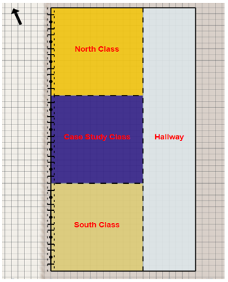
To enhance the model’s representativeness and reflect the real boundary conditions, the two adjacent classrooms—located respectively to the north and south—as well as the corridor, were also modeled. The spatial configuration is illustrated in Figure 1.
Figure 1. Model geometry
All external walls-oriented West were assigned the boundary condition: Outdoors. External walls facing South, East, and North were treated as adiabatic surfaces, representing thermal separation from adjacent zones assumed to be at the same temperature—therefore modeling a plane of thermal symmetry, as described in the EnergyPlus Engineering Reference [14].
All internal walls were assigned boundary conditions corresponding to the thermal zone sharing the respective surface.
Table 1 reports the geometrical dimensions of the modeled classroom.
The occupancy rate was defined to guarantee a minimum area of 2 m2 per person [15], with an occupancy schedule from 8:00 AM to 1:00 PM, Monday through Saturday, based on the data recorded by the installed sensor. Natural ventilation was modeled and activated exclusively during occupied periods. For the building envelope, glazed elements were represented as single-pane windows with 6 mm glass. Table 2 lists the thermal transmittances (U-values) of all opaque envelope components, with layers ordered from outside to inside.
Table 1. Model dimensions
|
Dimension |
Value |
Unit |
|
L |
7.50 |
m |
|
l |
7 |
m |
|
h |
3 |
m |
Table 2. Case study envelope
|
Layer |
U-value |
Unit |
|
Exterior wall |
1.29 |
W.m-2.K-1 |
|
Interior wall |
0.55 |
W.m-2.K-1 |
|
Roof |
0.20 |
W.m-2.K-1 |
|
Floor |
2.53 |
W.m-2.K-1 |
The external wall stratigraphy consists of prefabricated concrete panels with an external and internal plaster finish. Internal partitions are composed of two layers of gypsum board with a rock-wool panel sandwiched between them for acoustic insulation. The roof comprises a reinforced concrete slab with an air gap and acoustic-absorbent panels; during a recent retrofit, a 20 cm thermal insulation layer was added above the slab, and the entire roof surface was treated with a cool-roof coating. The floor-on-ground has a conventional, uninsulated concrete build-up finished with Gres.
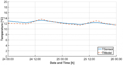
For model validation, a period during which the school was fully unoccupied, and the HVAC system was definitively switched off, was selected, thus eliminating the natural ventilation contribution, which would otherwise be difficult to estimate due to user-controlled operation. Analysis of the sensor data indicated that the ideal interval coincided with the Christmas holiday closure, specifically from 24 December to 25 December 2024. Hourly outdoor temperatures and solar radiation values were sourced from meteorological stations near Carpi via the ARPAE dext3r portal [16]. Figure 2 compares the internal temperature profiles obtained from the installed sensor measurements with those generated by the model simulation.
This comparison of internal temperatures yielded a mean error of 2.2%, with a maximum deviation of 6% over the simulation period.
These results were considered satisfactory; therefore, the model—maintaining the same geometry—was used to extend the study to a broader set of envelope configurations representative of the most common building typologies in the reference area. This choice is supported by the findings of Dongellini et al. [17] and aligned with the guidelines provided in the UNI/TR 11552 standard [18], which offers a catalogue of typical opaque building elements categorized by construction period and geographical area.
Figure 2. Indoor temperature comparison
For the windows, a double-glazing configuration with a 6/20/6 setup and an air gap was assumed. The thermal characteristics of the opaque components are presented in Table 3.
Table 3. S1 envelope
|
Layer |
U-value |
Unit |
|
Exterior wall |
1.83 |
W.m-2.K-1 |
|
Interior wall |
1.57 |
W.m-2.K-1 |
|
Roof |
1.96 |
W.m-2.K-1 |
|
Floor |
1.89 |
W.m-2.K-1 |
The scenario referred to as S1 represents the baseline condition of the existing building. It consists of 25 cm solid brick walls, a concrete floor slab, and a concrete floor finish with gres tiles.
This study also considers two additional retrofit scenarios:
(1) S2: Represents the most adopted envelope retrofit strategy in Italy in recent years-external insulation using a 14 cm rock-wool panel applied to the outer surface of the external walls.
(2) S3: Represents an internal insulation strategy, involving the application of a 4 cm rock-wool panel with a lightweight gypsum board finish on all internal surfaces, excluding the floor.
Rock-wool was assumed to have an effective thermal conductivity (λ) of 0.05 W.m-1.K-1 in all simulated scenarios.
The window configuration was kept identical across all three scenarios. The room occupancy was defined to guarantee a minimum area of 2 m2 per person [15], with an occupancy schedule set from Monday to Friday, 8:00 AM to 1:00 PM, followed by a one-hour lunch break and afternoon re-entry from 2:00 PM to 4:00 PM. The metabolic activity level of occupants was set to produce 100 W per person.
For ventilation, all scenarios assumed an air exchange rate compliant with the UNI EN 16798 standard [19], fixed at 7 L.s-1 per person. Internal loads were also assigned to account for equipment, assuming the presence of a computer and an interactive whiteboard.
Lighting loads were defined to meet the illuminance levels required by UNI EN 12464 [20]. The temperature setpoints were established at 20℃ for heating and 26℃ for cooling [2]. An ideal HVAC system was assumed at this stage to quantify the heating and cooling loads and energy demands associated with each envelope configuration.
Simulations for the three scenarios were run over the course of a full calendar year, considering school closures during holidays as well as the extended summer break.
The results highlight how S3 produced an environment with a higher thermal reactivity. The internal insulation applied to the envelope surfaces resulted in a very low thermal mass, making the indoor space more sensitive and responsive to changes in ambient conditions. This behavior is clearly illustrated in Figure 3, which displays the internal temperature profiles for all three scenarios. The graph refers to a Friday and a Saturday in January, corresponding to the heating season.
Scenarios S1 and S2 show similar trends, with S2 exhibiting a slight shift in the temperature curve due to the reduced U-value of the external wall, made possible by the added insulation.
The temperature profile of S3 demonstrates how, during occupied hours, the indoor environment reaches comfortable conditions faster than in the other two cases, potentially offering improved thermal comfort. The high responsiveness of S3 is particularly evident during weekend closures, where the indoor temperature reacts much more rapidly to increases in external temperature and solar gains compared to S1 and S2.
The extreme reactivity of the S3 envelope is further demonstrated in Figure 4, which shows the heating power profile over a typical school day in January. Here, too, the low thermal inertia of the S3 configuration, relative to S1 and S2, results in a substantially lower average power demand. Moreover, since the integral of the area under each power curve represents the total daily energy requirement, it can be asserted that S3 achieves tangible energy savings during the heating season.

Figure 3. Environmental response

Figure 4. Heating power
In both S1 and S2, the layers immediately adjacent to the indoor environment consist of construction materials characterized by high bulk density (ρ) and substantial thickness (t), resulting in a very large areal heat capacity Eq. (1).
$C_a=\rho c_p t$ (1)
This parameter quantifies the material’s capacity to store thermal energy and thus its resistance to rapid temperature fluctuations. Conversely, in S3 the layer facing the interior comprises 40 mm of rock-wool (low ρ) topped with a 5 mm lightweight gypsum board (low ρ), yielding a markedly reduced areal heat capacity and correspondingly faster thermal response.
Analysing the annual heating and cooling demands over the entire school period reveals that Scenario S2 achieves only a modest reduction in heating demand. In Scenario S3, however, with internal insulation applied to the walls and ceiling, heating demand falls to less than half that of the baseline.
The trade-off is that a highly reactive, low-inertia envelope introduces drawbacks on the cooling side. Figure 5 summarizes the heating and cooling demands for all three scenarios: S2 does not significantly increase cooling demand relative to S1—partly because the school closes in early June, thus avoiding the peak overheating period. In contrast, the low thermal inertia of S3 provokes overheating even during middle seasons, resulting in a cooling demand 1.7 times higher than in S1.
This heightened responsiveness leads to an extension of the cooling season also to spring and autumn and, consequently, to an increased cooling energy demand. Two principal factors drive this phenomenon: internal heat gains (people, given the high occupancy density typical of such spaces) and solar gains transmitted through extensive glazed areas via both direct and diffuse solar radiation.
Thus, to achieve an envelope that is both highly responsive—thereby maximizing overall energy savings—and capable of maintaining indoor thermal comfort, it is critical to mitigate the risk of overheating during the mid seasons. Since internal gains cannot be decreased, the definitive solution is the implementation of solar-shading systems, which minimize the thermal energy flux through fenestration.
For these reasons, an additional scenario (S4) is introduced in the study. This configuration is identical to S3 except for the incorporation of an in between-glass blind. By adjusting the slat angle, this device attenuates solar gains and mitigates the glare effect. A control strategy was defined whereby the blind closes automatically whenever incident solar irradiance at the site exceeds 300 W.m-2. This threshold was derived from the relevant UNI EN ISO 52016-1 [21], having been identified as the limit above which glare and excessive solar gain may occur within the occupied spaces.
Table 4 shows the technical specifications of the installed Venetian blinds.
The installation of the venetian blind within the glazing system leads to a reduction in thermal energy gain through the window components, from an annual total of 5840 kWh in scenario S3 to 4007 kWh in scenario S4. This corresponds to a percentage reduction of 31% compared to the pre-intervention case.
Figure 6 illustrates the thermal power per unit area entering the room through the glazing. The significant contribution of the installed device is evident, yielding a marked reduction in transmitted power throughout the year. However, it should be noted that solar gains are also reduced during the winter months, when they help to lower the heating load demand of the building. Consequently, there is a slight increase in heating demand and a substantially greater reduction in cooling demand, since these gains are of primary importance during the summer season.
Table 5 presents the annual heating and cooling demands for scenarios S3 and S4. The heating demand increases by only 33 kWh, while the cooling demand decreases by 131 kWh, resulting in an overall net reduction in energy demand.

Figure 5. Heating power

Figure 6. Solar gain comparison
Table 4. Blind technical specifications
|
Slat Orientation |
Horizontal |
|
Slat width |
0.015 m |
|
Slat separation |
0.02 m |
|
Slat thickness |
0.001 m |
|
Slat angle |
45 deg |
|
Slat conductivity |
160 W.m-1.K-1 |
|
Slat solar reflectance |
0.65 |
Table 5. Blind technical specifications
|
Scenario |
Heating |
Cooling |
Unit |
|
S3 |
732 |
555 |
kWh |
|
S4 |
765 |
424 |
kWh |
4.1 Centralized system vs. delocalized system
Most Italian school buildings are equipped with centralized heating systems. The boiler room typically houses a methane-fired condensing boiler and circulation pumps that distribute hot water through the distribution network to the terminal units; some systems also include tanks for domestic hot water. In the majority of buildings, the terminal units are radiators, which require very high supply-water temperatures (around 70℃) and therefore are not ideally matched with a condensing boiler, as they reduce its generation efficiency. These systems often exhibit significant inefficiencies, particularly in the distribution network: it is not uncommon for the pipes to date from the building’s original construction and to have severely degraded insulation, leading to distribution losses of up to 20%. From an HVAC perspective, very few schools have cooling systems, which causes severe discomfort due to overheating and compromised thermal comfort—one of the reasons why the school year is suspended for approximately three months every summer.
Another issue associated with a large, centralized plant is the complexity of control. Often, systems are started well in advance or remain in operation even when the spaces are unoccupied. These inefficiencies can considerably increase energy demand. Moreover, from an economic standpoint, the management and maintenance costs of such systems are high. For these reasons—within the framework of a building retrofit—besides the envelope measures discussed previously, it is crucial to improve plant efficiency. One viable strategy is the adoption of decentralized, independent systems capable of serving individual thermal zones with a very high level of control. This approach would raise distribution efficiency to an almost unity value and drastically reduce maintenance and management expenses. Furthermore, by implementing packaged heat pumps, full plant electrification could be achieved and operated in conjunction with an existing photovoltaic system, thereby increasing the share of renewable energy for building conditioning as required by Italian regulations [22, 23]. The installation of heat pumps would also satisfy the cooling demand of the building, enhance thermal comfort, and potentially allow for an extension of the academic calendar.
Deploying decentralized systems also facilitates a phased, zone-by-zone energy retrofit of the building. As a result, there is no need for extensive, high-cost construction sites—which often lead to operational shutdowns and disruptions, limited funding opportunities due to elevated project costs, and increased risk of work interruptions or delays that further compound inconvenience and expense.
Within the framework of a comprehensive retrofit of the proposed building, the annual energy demand has been analyzed for all scenarios. In S1, representing the baseline condition, a centralized system was assumed, comprising a methane-fired boiler for heating and, optionally, a chiller to meet any summer cooling load. Radiators were selected as the terminal units, and distribution losses were assumed to reflect the building’s original 1980s-era piping and degraded insulation. S2 retains the same system topology—since retrofit interventions rarely replace the entire plant, focusing instead on renewing only the generation components. In scenarios s3 and S4, however, a decentralized approach is introduced via a packaged heat pump (PHP). Equipment efficiencies were determined according to UNI/TS 11300‑2:2019 [24] and the age of the systems. For the chiller and the PHP in cooling mode, an average EER of 2.7 was assumed, while for the PHP in heating mode, a COP of 3.0 was used. Primary‑energy conversion factors for natural gas and electricity were taken from UNI/TS 11300-2019 [24] and set at 1.05 and 2.42, respectively. Table 6 reports the assumed plant efficiencies of S1 and S2.
Table 6. Plant efficiency
|
Efficiency |
S1-S2 |
S3-S4 |
|
ηg |
0.94/2.7 |
3.0/2.7 |
|
ηd |
0.9 |
1 |
|
ηr |
0.93 |
0.93 |
|
ηe |
0.94 |
0.9 |
For the estimation of the boiler's generation efficiency, a single stage condensing boiler was considered. For the distribution efficiency, reference was made to the UNI 10200 [25] standard, which indicates that for a centralized system with radiators and horizontal distribution dating back to the 1980s, the heat loss in the distribution network is 20%. Of this, 15% can be considered recovered by internal building components, thus contributing to winter space heating, while the remaining 5% are considered effective losses. In this study, an additional 5% of effective losses was factored in, attributed to the very common occurrence of damaged insulation. For the regulation efficiency, a single-zone control with a ±2℃ control band was assumed for all scenarios.
For the emission efficiency in scenarios S1 and S2, a radiator installed on an external wall in a room with a height below 4 m was considered. Conversely, for scenarios S3 and S4, the emission efficiency was considered equal to that of the unit's heat exchanger and was assumed to be 0.9.
In scenarios S1 and S2, this results in an overall efficiency of 74%, which can be considered a conservative figure compared to scenarios that exhibit much larger and more frequent losses in this sector.
Figure 7 illustrates the primary energy demand across the four scenarios. It is evident that the combined approach of internal insulation and a decentralized system results in a significant reduction in heating demand. Scenario S3, in contrast, shows a marked increase in cooling demand. The S4 solution provides a substantial decrease in winter heating demand while also lowering the cooling requirement compared to S3.

Figure 7. Primary energy demand
4.2 Natural ventilation vs. mechanical ventilation
As shown in the article by Stabile et al. [26], in which is evaluated the impact of a ventilation retrofit on classroom indoor air quality and space‑heating energy use is evaluated by comparing natural ventilation and a VMC system with heat recovery and CO₂ set point at 1000 ppm. This study demonstrates that longer natural airing reduced CO₂ but also allowed more outdoor sub-micron particles indoors. Mechanical ventilation-maintained CO₂ below 1000 ppm reliably.
Manual airing did not reduce indoor-generated PM₁₀ (ratios ≫ 1 remained unchanged). Mechanical ventilation lowered sub‑micron particle penetration (indoor‑to‑outdoor ratios of 0.39-0.56) and diluted super-micron PM₁₀ more effectively. Heat recovery in the mechanical system cut heating energy demand by 32% compared to the manual‑airing ventilation rate required by standards.
In this study, the CO₂ concentration measured in the classroom used for model validation is compared with the concentration profile that would occur over a typical school day under a controlled mechanical ventilation system. The ventilation rate for the mechanical‐ventilation scenario was calculated according to UNI EN 16798‑1:2019 [19] and set at 7 L.s-1 per person. The two concentration curves are shown in Figure 8.

Figure 8. CO2 concentration
As clearly shown in Figure 8, under natural ventilation CO₂ concentrations peak at around 3000 ppm, compared with the 1000 ppm threshold above which comfort—and, over the long term, health—issues may arise according to the World Health Organization. The sharp drops in CO₂ during the morning indicate likely window openings, which momentarily flush the air; once closed again, however, high occupancy drives CO₂ back up to roughly 3000 ppm. By contrast, a demand‑controlled mechanical ventilation system maintains CO₂ at the 1000 ppm threshold throughout the entire school day.
An additional benefit of mechanical ventilation—subject of future detailed studies—is the ability to install a heat exchanger. In winter, this can pre‑warm incoming fresh air by recovering heat from the exhaust stream. In summer, it permits free‑cooling when outdoor temperatures are lower than indoors or reduces supply‑air temperature when outdoor air is warmer. The winter case is especially advantageous owing to the larger temperature difference between inside and outside. In a classroom environment—where hourly air changes can reach 3.5 volumes per hour—heat recovery could yield a substantial reduction in heating demand: indeed, the CO₂ study reports energy savings of approximately 32% for space heating.
4.3 Thermal comfort
To determine which of the four proposed scenarios provides the best indoor environment in terms of thermal comfort, the operative temperature was first calculated as described in Eq. (2).
$T_{o p}=\frac{h_c T_a+h_r T_{m r}}{h_c+h_r}$ (2)
Operative temperature is a key metric in assessing thermal comfort as it provides a more holistic measure of how an individual perceives the thermal environment.
Essentially, operative temperature effectively combines the influence of air temperature and mean radiant temperature (the average temperature of the surrounding surfaces) into a single value, offering a more accurate indication of a person's thermal sensation and overall comfort than air temperature alone.
Subsequently, an analysis was carried out—limited to periods when the building is occupied—by counting the number of hours falling within different operative temperature ranges.

Figure 9. Operative temperature range
Figure 9 shows that Scenarios S1 and S2 have the highest number of hours in the <17℃ range, whereas S3 and S4 record significantly fewer, thanks to the high responsiveness of the building envelope. A similar trend is observed in the 17–20℃ range.
In the optimal temperature range of 20–26℃, a progressive increase in the number of comfortable hours is evident, with S4 achieving the highest value. The difference between S3 and S4 in this ideal range can be attributed to the overheating periods: S4, benefiting from solar shading devices, significantly reduces the time spent in excessive operative temperature conditions.
This analysis further confirms that combining internal insulation with solar shading not only decreases thermal discomfort during winter but also limits overheating during warmer periods.
In this study, a dynamic energy analysis was performed using the EnergyPlus simulation software. The case study was used to validate the model and then employ it as a basis for a more general and extensive study of typical Italian school classrooms. Various scenarios were investigated, and it was highlighted that, for buildings with these characteristics: high internal gains, intermittent use, and large windows, the solution with internal insulation and solar shading is advantageous both from the perspective of primary energy reduction and thermal comfort. The importance of controlled mechanical ventilation was also emphasized, demonstrating how it enables a decrease in indoor CO2 concentration, ensuring greater comfort and facilitating the installation of a heat recovery unit that can further reduce energy demand. Furthermore, it was shown that in intermittently used buildings, the transient state and dynamic aspects are of significant importance, as are the complex interactions between the variables involved. This study highlights the necessity of a holistic approach during building retrofits, where the inertia of the building envelope plays a primary role within the set of variables.
|
Ca |
areal heat capacity, J.m-2.K-1 |
|
cp |
specific heat at constant pressure, J.kg-1.K-1 |
|
h |
room height, m |
|
L |
west/east side wall length, m |
|
l |
north/south side wall length, m |
|
t |
thickness, m |
|
U |
global heat transfer coefficient, W.m-2.K-1 |
|
Greek symbols |
|
|
ηd |
distribution efficiency |
|
ηe |
emission efficiency |
|
ηg |
generation efficiency |
|
ηr |
regulation efficiency |
|
$\lambda$ |
thermal conductivity, W.m-1.K-1 |
|
$\rho$ |
density, kg.m-3 |
|
Subscripts |
|
|
ARPAE |
Agenzia Regionale per la Prevenzione, l’Ambiente e l’Energia |
|
COP |
coefficient of performance |
|
EER |
energy efficency ratio |
|
HVAC |
Heating, Ventilation and Air Conditioning |
|
PHP |
packaged heat pump |
|
S1 |
Scenario 1 |
|
S2 |
Scenario 2 |
|
S3 |
Scenario 3 |
|
S4 |
Scenario 4 |
|
SCFs |
solar control films |
[1] IEA, IRENA & UN Climate Change High-Level Champions (2023). Breakthrough Agenda Report 2023. IEA, Paris. https://www.iea.org/reports/breakthrough-agenda-report-2023.
[2] UNI/TS 11300‑1:2014. Prestazioni energetiche degli edifici – Parte 1: Determinazione del fabbisogno di energia termica dell’edificio per la climatizzazione estiva ed invernale. Ente Italiano di Normazione, Milano.
[3] Zakula, T., Bagaric, M., Ferdelji, N., Milovanovic, B., Mudrinic, S., Ritosa, K. (2019). Comparison of dynamic simulations and the ISO 52016 standard for the assessment of building energy performance. Applied Energy, 254: 113553. https://doi.org/10.1016/j.apenergy.2019.113553
[4] Calise, F., Cappiello, F.L., Cimmino, L., Vicidomini, M. (2024). Semi-stationary and dynamic simulation models: A critical comparison of the energy and economic savings for the energy refurbishment of buildings. Energy, 300: 131618. https://doi.org/10.1016/j.energy.2024.131618
[5] Hu, C., Xu, R., Meng, X. (2022). A systemic review to improve the intermittent operation efficiency of air-conditioning and heating system. Journal of Building Engineering, 60: 105136. https://doi.org/10.1016/j.jobe.2022.105136
[6] Verbeke, S., Audenaert, A. (2018). Thermal inertia in buildings: A review of impacts across climate and building use. Renewable and Sustainable Energy Reviews, 82: 2300-2318. https://doi.org/10.1016/j.rser.2017.08.083
[7] Meng, X., Huang, Y., Cao, Y., Gao, Y., Hou, C., Zhang, L., Shen, Q. (2018). Optimization of the wall thermal insulation characteristics based on the intermittent heating operation. Case Studies in Construction Materials, 9: e00188. https://doi.org/10.1016/j.cscm.2018.e00188
[8] Meng, X., Luo, T., Gao, Y., Zhang, L., et al. (2018). Comparative analysis on thermal performance of different wall insulation forms under the air-conditioning intermittent operation in summer. Applied Thermal Engineering, 130: 429-438. https://doi.org/10.1016/j.applthermaleng.2017.11.042
[9] Yuan, L., Kang, Y., Wang, S., Zhong, K. (2017). Effects of thermal insulation characteristics on energy consumption of buildings with intermittently operated air-conditioning systems under real time varying climate conditions. Energy and Buildings, 155: 559-570. https://doi.org/10.1016/j.enbuild.2017.09.012
[10] Zhou, J., Li, Y., Xiao, X., Long, E. (2017). Experimental research on thermal performance differences of building envelopes in multiple heating operation conditions. Procedia Engineering, 205: 628-635. https://doi.org/10.1016/j.proeng.2017.10.409.
[11] Bojić, M.L., Loveday, D.L. (1997). The influence on building thermal behavior of the insulation/masonry distribution in a three-layered construction. Energy and Buildings, 26(2): 153-157. https://doi.org/10.1016/S0378-7788(96)01029-8
[12] Pereira, J., Teixeira, H., Gomes, M.D.G., Moret Rodrigues, A. (2022). Performance of solar control films on building glazing: A literature review. Applied Sciences, 12(12): 5923. https://doi.org/10.3390/app12125923
[13] Mainini, A.G., Bonato, D., Poli, T., Speroni, A. (2015). Lean strategies for window retrofit of Italian office buildings: Impact on energy use, thermal and visual comfort. Energy Procedia, 70: 719-728. https://doi.org/10.1016/j.egypro.2015.02.181
[14] U.S. Department of Energy (2022). EnergyPlus™ Version 22.1.0 Documentation - Engineering reference, Build ed759b17ee. https://energyplus.net/assets/nrel_custom/pdfs/pdfs_v22.1.0/EngineeringReference.pdf.
[15] Decreto Ministeriale. (1975). Norme tecniche aggiornate relative all’edilizia scolastica, ivi compresi gli indici minimi di funzionalità didattica, edilizia ed urbanistica. Supplemento ordinario alla Gazzetta Ufficiale, n. 29, 2 febbraio 1976.
[16] ARPAE Emilia‑Romagna. Dext3r: Webapp di estrazione dati di Arpae SIMC. https://simc.arpae.it/dext3r/.
[17] Dongellini, M., Abbenante, M., Morini, G.L. (2016). Energy performance assessment of the heating system refurbishment on a school building in Modena, Italy. Energy Procedia, 101: 948-955. https://doi.org/10.1016/j.egypro.2016.11.120
[18] UNI/TR 11552:2014. Abaco delle strutture costituenti l’involucro opaco degli edifici - Parametri termo‑fisici. Ente Nazionale Italiano di Unificazione (UNI), Milano.
[19] UNI EN 16798‑1:2019. Prestazione energetica degli edifici – Ventilazione per gli edifici – Parte 1: Parametri di ingresso dell’ambiente interno per la progettazione e la valutazione della prestazione energetica degli edifici in relazione alla qualità dell’aria interna, all’ambiente termico, all’illuminazione e all’acustica, Ente Nazionale Italiano di Unificazione (UNI), Milano. https://store.uni.com/en/uni-en-16798-1-2019.
[20] UNI EN 12464‑1:2011. Light and lighting – Lighting of work places – Part 1: Indoor work places. Ente Nazionale Italiano di Unificazione (UNI), Milano. https://www.iso.org/standard/56165.html.
[21] UNI EN ISO 52016‑1:2017. Prestazione energetica degli edifici – Fabbisogni di energia per riscaldamento e raffrescamento, temperature interne e carichi termici sensibili e latenti – Parte 1: Procedure di calcolo. Ente Nazionale Italiano di Unificazione (UNI), Milano. https://www.iso.org/standard/65696.html.
[22] Ministero dello Sviluppo Economico. (2015). Decreto interministeriale 26 giugno 2015 – Applicazione delle metodologie di calcolo delle prestazioni energetiche e definizione delle prescrizioni e dei requisiti minimi degli edifici. Gazzetta Ufficiale Serie Generale, n. 162, Suppl.Ordinario n. 39. https://www.gazzettaufficiale.it/atto/serie_generale/caricaDettaglioAtto/originario?atto.codiceRedazionale=15A05198&atto.dataPubblicazioneGazzetta=2015-07-15.
[23] Decreto Legislativo 8 novembre 2021, n. 199. Attuazione della direttiva (UE) 2018/2001 del Parlamento europeo e del Consiglio, dell’11 dicembre 2018, sulla promozione dell’uso dell’energia da fonti rinnovabili. Gazzetta Ufficiale Serie Generale, n. 285, Suppl. Ordinario n. 42/L. https://www.gazzettaufficiale.it/eli/id/2021/11/30/21G00214/sg.
[24] UNI/TS 11300‑2:2019. Prestazioni energetiche degli edifici – Parte 2: Determinazione del fabbisogno di energia primaria e dei rendimenti per la climatizzazione invernale, per la produzione di acqua calda sanitaria, per la ventilazione e per l’illuminazione in edifici non residenziali. Ente Italiano di Unificazione (UNI), Milano. https://store.uni.com/uni/uni-ts-11300-2-2019.
[25] UNI 10200:2018. Impianti termici centralizzati di climatizzazione invernale ed estiva e di produzione di acqua calda sanitaria – Criteri di progettazione, esercizio e contabilizzazione dei consumi di energia termica, Ente Italiano di Normazione (UNI), Milano. https://store.uni.com/uni-10200-2018.
[26] Stabile, L., Buonanno, G., Frattolillo, A., Dell’Isola, M. (2019). The effect of the ventilation retrofit in a school on CO2, airborne particles, and energy consumptions. Building and Environment, 156: 1-11. https://doi.org/10.1016/j.buildenv.2019.04.001