Dennis Navarrete Ttito*![]() | Dany Quispe Suarez
| Dany Quispe Suarez![]() | Jorge Apaza Gutierrez
| Jorge Apaza Gutierrez![]() | Waygand Beltran Quispe
| Waygand Beltran Quispe![]() | Paul Pinto Carpio
| Paul Pinto Carpio![]() | Christofer Diaz Arapa
| Christofer Diaz Arapa![]()
© 2025 The authors. This article is published by IIETA and is licensed under the CC BY 4.0 license (http://creativecommons.org/licenses/by/4.0/).
OPEN ACCESS
This study computationally develops and evaluates an air duct system designed to reduce hot gas recirculation within the engine compartment of a pickup truck (Toyota Hilux 2022), aiming to improve the thermal behavior of the underhood cooling system under low-speed urban and highway conditions. Two aerodynamic ducts (Design A and Design B) were created using 3D modeling in SolidWorks and analyzed through CFD simulations in ANSYS CFX with the k–ε turbulence model. Subsonic inlet conditions of 2.78 m/s (urban, 10 km/h) and 33.33 m/s (highway, 120 km/h) were defined to represent urban and highway environments. Design A exhibited a better outlet velocity distribution, while Design B showed internal pressure accumulations exceeding 6000 Pa due to higher geometric complexity. Based on these results, Design A was selected for further thermal and structural evaluation. A transient heat transfer study was conducted using ANSYS CFX, with detailed meshing of the engine, radiator, and duct. Additionally, MATLAB was used to validate convective heat transfer calculations at the duct outlet. A maximum temperature reduction of 7.22℃ was achieved at the engine’s rear zone at 120 km/h. These results support the integration of low-profile frontal ducts to enhance thermal evacuation without major vehicle modifications.
thermal recirculation, front duct design, CFD simulation, heat transfer analysis, engine cooling, Ansys CFX, Automotive thermal optimization
One of the most relevant current challenges in automotive engineering is the thermal optimization of the engine compartment, particularly the management of airflow under low-speed urban conditions. In these scenarios, which are highly characteristic of dense urban traffic [1], the amount of fresh air entering through the vehicle's front grille is significantly reduced [2]. This situation, combined with the heat generated by the engine's operation, creates a critical environment where hot gases become trapped within the underhood region. This phenomenon, known as hot air recirculation, drastically elevates the temperature in critical areas and compromises the efficiency of the entire cooling system. Components such as exhaust manifolds, turbochargers, and electronic control units are subjected to severe thermal loads, which can lead to premature degradation.
This issue is further compounded by the fact that the internal combustion process is inherently inefficient. It is estimated that a substantial portion of the energy generated by the engine, between 30% and 35%, is lost as heat [3]. Consequently, any inadequacy in thermal management not only affects the durability and operational lifespan of the components but also directly impacts the overall performance and reliability of the propulsion system [4]. For this reason, addressing the problem of hot air recirculation is not just a matter of component longevity; it is a fundamental aspect of modern vehicle design aimed at maximizing efficiency and safety in demanding operational conditions.
To address the challenge of hot gas accumulation and recirculation within the engine compartment, various technologies have been developed. Among them, the use of strategically designed and directed air ducts has proven to be one of the most effective solutions. For instance, Song et al. [5] demonstrated that targeted airflow channeling can significantly reduce underhood hot air retention and improve the evacuation of heated gases from critical areas. In the industry, models such as the Ford F-150 have adopted active grille systems and optimized front-end geometries to reduce cooling drag and enhance heat dissipation under real driving conditions [6]. Likewise, studies by Zhao et al. [7] and Franzke et al. [8] have shown that geometric optimization of airflow paths, whether through sealed guides, ducting, or upstream flow modifications, can reduce localized heat stagnation, improve ventilation rates, and stabilize component temperatures during high-load or low-speed urban operation.
The relevance of this approach lies in its ability to prevent thermal hotspots, extend the operational life of engine components, and maintain optimal performance even in demanding driving environments. In the context of modern automotive engineering, enhanced airflow management through ducting is a key strategy for improving underhood thermal balance, particularly in vehicles exposed to high ambient temperatures or prolonged urban traffic conditions. Therefore, establishing a reliable and replicable methodology to identify, quantify, and mitigate the hot air recirculation phenomenon from the early design stages is essential.
Recent advances in three-dimensional modeling (CAD) and Computational Fluid Dynamics (CFD) [9] simulation have proven to be robust tools for accurately predicting thermal behavior in critical engine compartment zones, even under low-speed conditions, where the flow of fresh air is significantly reduced [10]. This approach has been validated in studies that combine virtual modeling with experimental correlation, demonstrating its usefulness in evaluating passive air guiding strategies and identifying recirculation zones that may not be apparent in conventional physical testing [11]. Unlike traditional methods that rely on physical prototypes and high-cost, time-consuming experimental campaigns, virtual environments enable faster iterative exploration, allowing for data-driven design decisions based on replicable numerical results. Additionally, the use of parametric models in CFD allows for the efficient evaluation of multiple geometric configurations, which is particularly valuable in projects with time and resource constraints [12].
In this context, the present research is aimed at designing and computationally evaluating an air duct system that reduces the accumulation and recirculation of hot gases within the engine compartment. Three-dimensional CAD modeling and CFD simulation were used to address this challenge [9]. The methodology is structured in several key stages: First, the thermal and aerodynamic behavior of the base model of a Toyota Hilux without ducts will be simulated to establish a reference temperature of 105℃ in the engine and to identify critical zones of air recirculation. Subsequently, two duct designs, named Design A and Design B, will be proposed and modeled. These ducts originate in the vehicle's front fog lights, are directed in an arched shape to avoid the tires, and guide the fresh airflow toward the rear of the engine [13]. The main objective of this configuration is to direct a jet of cool air downward to promote the evacuation of hot gases trapped in the engine bay. Both designs will be compared to determine which one presents a higher air outflow velocity, a key indicator of its effectiveness. The most suitable design will be selected for the next phase: a detailed simulation that integrates the engine's heat transfer and airflow. Using a combination of data from CFD (ANSYS) and heat transfer analysis (MATLAB), temperature variations on the engine's contour will be quantified based on the ducts' impact area and different air intake velocities. The results of this study will strengthen thermal management strategies in urban low-speed scenarios and establish a reproducible framework for future design iterations, with potential impact on the reliability and performance of the propulsion system.
This research adopted a computational approach supported by studies that have validated the combined use of CFD simulations and simplified thermal analysis techniques to understand hot air recirculation and its impact on the underhood cooling system under urban traffic conditions [5, 14].
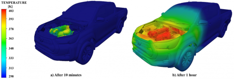
To analyze the thermal behavior of the engine compartment over different operating periods, a transient study was developed using ANSYS CFX, based on a realistic three-dimensional geometry of a 2022 Toyota Hilux. The initial and boundary temperature conditions were configured according to the values reported in the manufacturer’s technical manual and reliable data from the automotive sector [15].
Figure 1 illustrates two simulated scenarios: (a) after 10 minutes of engine operation, and (b) after 1 hour of continuous operation. These simulations revealed the surface temperature distribution in critical engine components such as the cylinder head, engine sides, exhaust area, and radiator.
Figure 1. Thermal evolution of Hilux: a) 10 Minutes, b) 1 Hour
Table 1. Typical temperature ranges of engine components and their sources
|
Vehicle Component |
Value |
Source / Comment |
|
Top of the engine (cylinder head, cover) |
80 – 105 |
Toyota repair manual, recent CFD studies |
|
Engine block housing |
70 – 100 |
Thermal engineering manuals, ANSYS simulation |
|
Front radiator zone (air intake) |
45 – 70 |
CFD results, experimental cooling data |
|
Radiator inlet (liquid coolant) |
45 – 65 |
Toyota technical manual, normal operating conditions |
|
Sides of the engine (structure and mounts) |
70 – 105 |
Reference thermal models, structural analysis |
|
Rear engine area (exhaust zone) |
75 – 105 |
High thermal loads from exhaust gases, validated analysis |
|
Outer surface of the engine block |
50 – 90 |
Field studies and thermographic tests |
|
Engine base (near oil pan) |
60 – 90 |
Estimated oil temperature, conductive heat transfer |
The model considered heat transfer by convection and conduction, in addition to the effect of fan-induced flow [16]. This approach has been used in previous studies, confirming the effectiveness of CFD tools to visualize heat accumulation, evaluate critical temperature conditions, and propose strategies for more efficient thermal evacuation [10, 17].
To facilitate the understanding of the thermal analysis, Table 1 was prepared based on technical information from manuals and official Toyota documentation [18]. These data served as the basis for the simulations conducted in ANSYS CFX, aiming to evaluate temperature behavior under steady-state conditions and analyze the heating of areas adjacent to the engine. A maximum temperature of 378 K was considered, corresponding to the normal operating conditions of a pickup truck under regular use. Although in the exceptional cases in which the surface temperature can reach up to 403 K due to cooling system failures or other overheating causes, the technical literature and manufacturer recommendations indicate a stable operating range between 373 K and 378 K.
2.1 Design, sizing, and preparation of ducts
Two three-dimensional designs (Designs A and Design B) were developed in SolidWorks, adapted to the available space behind the fog lights of a 2022 Toyota Hilux [18].
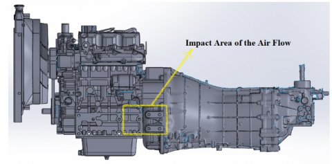
Real dimensions and structural constraints of the front compartment were respected to ensure physical compatibility and to avoid interference with other components. The region where the airflow impacts the engine surface is shown below, as defined in Figure 2.
Figure 2. Flow impact area at the duct outlet
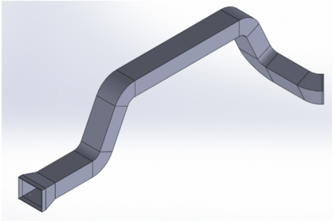
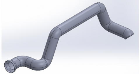
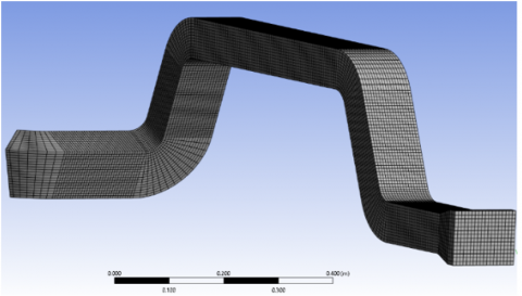
Two inverted “Z”-shaped designs (660 mm) were created with smooth transitions to reduce pressure losses and optimize unused space inside the vehicle (Figure 3).
However, in the area adjacent to the suspension, a critical decision had to be made regarding whether the routing would follow an internal or external path relative to it, ensuring sufficient clearance between the chassis and the tire without restricting its movement.
In the case of Design A, which features minimal directional changes, a square profile was selected to maximize airflow and efficiently utilize the available area.
The duct design was based on carefully defined geometric parameters. The total height of the inlet profile was 126 mm, measured from the bottom to the top edge in the side view, which defines the visible front contour. The inlet width progressively narrowed from 100 mm (top) to 74 mm (bottom), promoting flow acceleration. The front section, including its initial narrowing, is 90 mm long, ensuring efficient frontal air capture as it directs airflow toward the fender liner area.
The first ascending diagonal measured 260 mm in height, designed to avoid interference with the front tire by positioning the duct above the clearance space between the tire and the chassis. In the top view, the inlet depth from the front plane to the first bend of the duct measured 330 mm. The second diagonal (descending) measured 250 mm in height, allowing the duct to be routed above the structural level of the chassis support. The inlet-to-outlet section is 280 mm long, allowing the airflow to stabilize before the final curvature. In the case of Design B, this outlet featured a curvature radius of 30 mm, strategically oriented toward the underside of the vehicle to aid in the evacuation of hot air from the thermal compartment.
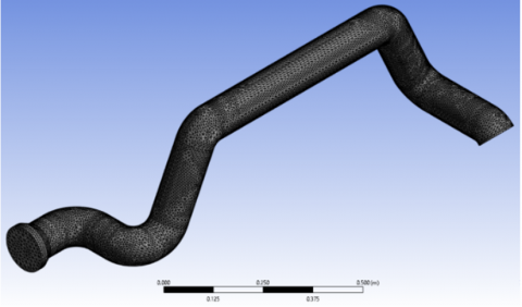
Design B, which incorporated multiple 90° bends, required the adoption of a circular profile due to its smooth transition between curvature changes. This also minimized welded joints or couplings during manufacturing, regardless of the selected material.
Both models were exported as closed solids for aerodynamic analysis via CFD simulation. To determine the performance of both duct designs, CFD simulations were conducted under identical conditions, considering vehicle speeds of 2.78 m/s and 33.33 m/s.
To ensure proper resolution of flow characteristics within ducts A and B, a structured mesh was implemented for both designs. Given the range of inlet velocities (2.78 m/s to 33.33 m/s), a refined tetrahedral mesh was used in wall-adjacent zones of Design A, while for Design B, which features a circular geometry, a shell-type mesh was employed, as it was easier to generate in such regions (Figure 4). Element size was adjusted to strike a balance between computational cost and the fidelity required to capture phenomena such as recirculation zones, pressure losses, and vortex formations. This approach is consistent with recommended practices in the technical literature, which emphasize the importance of mesh refinement in areas with high gradients and the use of adaptive techniques to maintain accuracy without significantly increasing computational cost [19].
In Table 2, the mesh refinement analysis conducted for Models A and B enabled the identification of the stabilization threshold for the variable of interest (maximum flow velocity), ensuring the numerical reliability of the CFD simulations. For Model A, the relative variation between consecutive simulations progressively decreased, reaching a difference below 0.1% from approximately 2 million elements (Simulation A5). Similarly, Model B showed clear stabilization starting at 1.7 million elements (Simulation B6).
Table 2. Properties of the boundary conditions of the refrigeration system
|
Design |
SIM |
Elements |
V max (m/s) |
% Difference |
|
A |
1 |
76,104 |
8.698 |
– |
|
2 |
129,778 |
7.61 |
12.49% |
|
|
3 |
261,800 |
7.969 |
4.72% |
|
|
4 |
632,664 |
7.995 |
0.33% |
|
|
5 |
2,117,664 |
8 |
0.06% |
|
|
6 |
5,505,926 |
8.002 |
0.03% |
|
|
B |
7 |
11,562,445 |
8.003 |
0.01% |
|
1 |
84,606 |
9.317 |
– |
|
|
2 |
118,421 |
9.445 |
1.37% |
|
|
3 |
200,286 |
9.498 |
0.56% |
|
|
4 |
371,987 |
9.54 |
0.44% |
|
|
5 |
890,042 |
9.579 |
0.41% |
|
|
6 |
1,780,145 |
9.595 |
0.17% |
|
|
7 |
3,200,000 |
9.602 |
0.07% |
These results indicate that both models achieve mesh-independent convergence at these discretization levels; thus, using a mesh with over 2 million elements represents a suitable compromise between numerical accuracy and computational cost. This step is essential to ensure that the differences observed between duct configurations are due to geometric conditions rather than errors caused by insufficient mesh resolution.
It should be noted that the effects of active grille shutters and PWM-controlled fans were not included in the present model, as the focus was restricted to passive duct geometries. Future studies should incorporate these elements to better capture their influence on flow distribution and hot air recirculation.
The CFD simulations were carried out in ANSYS CFX using the SST k-ω turbulence model, which is well-suited for capturing velocity gradients and dissipation near walls in confined flows. Operating conditions at 2.78 m/s (representing low-speed urban traffic) and 33.33 m/s (representing highway driving) were evaluated, defining uniform flow inlets, no-slip conditions on walls, and ambient pressure outlets [10, 17]. Although idle corresponds to 0 m/s with fan-dominated flow, the present study focused on low-speed free-stream conditions (2.78 m/s) to ensure airflow interaction with the ducts.
Table 3 summarizes the boundary conditions assigned at the nozzle inlet for both simulation cases, corresponding to low and high speeds. Relevant parameters such as flow regime, inlet velocity, turbulence model, and fluid properties are detailed, which were essential to ensure consistency in the comparison of results between both scenarios.
Table 3. Inlet boundary conditions at the nozzle
|
Parameter |
Case 1: Low Speed |
Case 2: High Speed |
Unit |
|
Flow regime |
Subsonic |
Subsonic |
– |
|
Inlet velocity |
2.78 |
33.33 |
m/s |
|
Turbulence model |
k–ε (standard k– epsilon) |
k–ε (standard k– epsilon) |
– |
|
Turbulent kinetic energy (k) |
0.05 |
0.05 |
m²/s² |
|
Turbulent dissipation rate (ε) |
0.10 |
0.10 |
m²/s³ |
|
Fluid static temperature |
298 |
298 |
K |
Specifically, the inlet was configured as subsonic flow with two representative velocity scenarios: one at 2.78 m/s (low-speed urban traffic) and another at 33.33 m/s (highway driving), corresponding to urban and highway conditions, respectively. For the simulation, the k–ε turbulence model was employed, widely used in automotive analyses for its balance between accuracy and computational efficiency. This model has shown good performance in CFD underhood studies, where it is necessary to reliably capture turbulence effects in complex geometries without incurring high computational cost [20]. Key parameters such as turbulent kinetic energy (k = 0.05 m²/s²), turbulent dissipation (ε = 0.1 m²/s³), and the static flow temperature (298 K) were defined as boundary conditions at the inlet [21].
Continuity:
$\frac{\partial\left(\rho u_j\right)}{\partial x_i}=0$ (1)
and the momentum equations are expressed by:
$\frac{\partial\left(\rho u_i u_j\right)}{\partial x_i}=-\frac{\partial p}{\partial x_i}+\frac{\partial}{\partial x_i}\left[\left(\mu+\mu_t\right)\left(\frac{\partial u_i}{\partial x_j}+\frac{\partial u_j}{\partial x_i}\right)\right]+\rho g_i$ (2)
Energy (enthalpy form):
$\rho c_p u_j \frac{\partial T}{\partial x_i}=\frac{\partial}{\partial x_i}\left[\left(\lambda+\lambda_t\right) \frac{\partial T}{\partial x_i}\right]+S_T$ (3)
k-equation:
$\frac{\partial\left(\rho k u_j\right)}{\partial x_i}=\frac{\partial}{\partial x_i}\left[\left(\mu+\frac{\mu_t}{\sigma_k}\right) \frac{\partial k}{\partial x_i}\right]+P_k-\rho \varepsilon$ (4)
$\varepsilon$-equation:
$\frac{\partial\left(\rho \varepsilon u_j\right)}{\partial x_i}=\frac{\partial}{\partial x_i}\left[\left(\mu+\frac{\mu_t}{\sigma_{\varepsilon}}\right) \frac{\partial \varepsilon}{\partial x_i}\right]+C_{\varepsilon 1} \frac{\varepsilon}{k} P_k-C_{\varepsilon 2} \rho \frac{\varepsilon^2}{k}$ (5)
Turbulent viscocity:
$\mu_t=\rho C_\mu \frac{k^2}{\varepsilon}$ (6)
Turbulent thermal conductivity:
$\lambda_t=\frac{\mu_t c_p}{P r_t}$ (7)
To ensure a comprehensive analysis, the engine and radiator were also modeled in ANSYS to enable subsequent evaluations both through applied calculations in MATLAB, using the aforementioned heat transfer and fluid dynamics equations, and through CFD simulations in ANSYS CFX [22]. The goal is to establish a reliable comparison between analytical and numerical results. Initially, the objective is to achieve stable outcomes by leveraging the meshing strategies previously discussed. Although the mesh refinement was specifically applied to the ducts, it serves a critical role in identifying which design better fulfills the purpose outlined in the introduction: enhancing the recirculation of hot gases.
To assess this, the outlet velocity of both ducts must be quantified, along with the pressure they exert on the duct walls, which translates into mechanical loads on the vehicle's mounting structures. This evaluation also contributes to identifying which design imposes lower structural loads on the vehicle chassis. Once the optimal duct configuration is selected based on these criteria, a coupled thermal-fluid analysis will be performed including the engine and radiator.
This will determine the heat transfer behavior at vehicle speeds of 2.78, 8.33, 13.89, 22.22, and 33.33 m/s (equivalent to 10, 30, 50, 80, and 120 km/h), enabling the quantification of the thermal differential (ΔT) introduced by the duct system under realistic operating conditions.
However, it should be emphasized that the structural evaluation was restricted to aerodynamic loading and did not include long-term material degradation phenomena. In particular, PP+GF composites commonly used in bumper and duct systems have a continuous-use temperature limit of approximately 90℃, which is lower than the 105℃ zones identified in the present simulations. Therefore, future studies should include creep and fatigue assessments under combined thermal and pressure loads to fully validate the durability of the solution.
2.2 Meshing and preparation of the engine and radiator
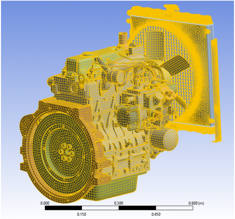
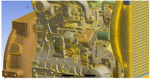
The engine, like the Toyota Hilux pickup truck, was not modeled as a traditional solid but was developed from STL files obtained through 3D scanning. This format poses significant challenges for meshing in CFD-dedicated software due to the high number of generated surfaces. To enable its analysis, the geometries were cleaned and smoothed using SolidWorks and later ANSYS Discovery. The truck model alone exceeded 5 million surfaces, while the engine surpassed 2.3 million, without accounting for the additional complexity introduced by the internal hood compartment, which significantly increased the surface count.
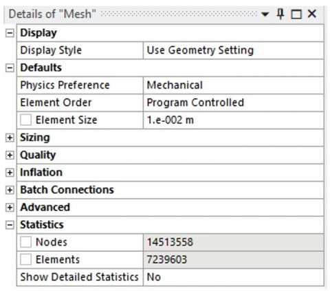
Once the surfaces were optimized in Discovery, the engine model was exported in STEP format, allowing for better integration into ANSYS meshing module. There, a mesh consisting of 7,239,603 elements was generated (Figure 5), pushing the limits of the computing system used (Intel Core i9 processor with 32 GB of RAM). Figure 6 presents representative details of the final engine mesh.
To evaluate the thermal performance of the selected duct, the analysis of convective heat exchange generated by the impact of the airflow on the thermal modules was considered [23]. This phenomenon can be described using the classical equations for forced convection heat transfer, which make it possible to quantify the heat flux transferred from the air to the impacted component [24]. Their application enables a quantitative assessment of the effectiveness of the proposed solution with the redesigned ducts [21, 23].
The air properties are required for the calculation of the dimensionless parameters and the convective coefficient. These properties are evaluated at a mean temperature close to that of the air jet [25, 26]. The expressions are:
Air density $(\rho)$:
$\rho=\frac{P}{(R . T)}$ (8)
Dynamic viscosity of air $(\mu)$:
$\mu=\mu_0 \cdot\left(\frac{T}{T_0}\right)^{\frac{3}{2}} \cdot \frac{\left(T_0+C\right)}{(T+C)}$ (9)
The Prandtl number was used as a parameter relating momentum diffusion to heat diffusion. It is defined as:
$\operatorname{Pr}=\frac{c_p \cdot \mu}{k}$ (10)
Thermal conductivity of air (k):
$k=k_0+k_1 T+k_2 T^2$ (11)
where, $c_p$ is the specific heat of air at constant pressure $\frac{{J}}{{kg} \cdot . {K}}$, $\mu$ the dynamic viscosity of air Pa.s and $k$ the thermal conductivity of air $\frac{W}{m \cdot K}[27,28]$.
$R e=\frac{\rho \cdot U \cdot D}{\mu}$ (12)
where, $\rho$ represents the air density $\frac{{kg}}{{m}^3}, U$ the mean flow velocity $\frac{m}{s}, D$ the hydraulic diameter of the duct $m$, and $\mu$ the dynamic viscosity of air [29, 30].
The Nusselt number was used as the dimensionless parameter relating convective heat transfer to conductive heat transfer within the fluid [28, 31], defined as:
$N u=\frac{h_{ {convection}} \cdot D}{k}$ (13)
where, $h_{\text {convection }}$ is the convective heat transfer coefficient $\frac{W}{m^2 \cdot K}, D$ the hydraulic diameter of the duct $m$, and $k$ the thermal conductivity of air $\frac{W}{m . K}$.
This number allows the evaluation of the efficiency with which heat is transferred from the duct walls to the air flow or vice versa [21]. Its value depends on the flow regime (laminar or turbulent), the thermophysical properties of the air, and the duct geometry. For internal flows with well-defined conditions, widely accepted empirical correlations exist to estimate the Nusselt number as a function of the Reynolds and Prandtl numbers.
The convective heat transfer coefficient h represents the ability of the air flow to transfer heat from the engine surface to the environment or vice versa. It is calculated from the Nusselt number by the expression:
$h=\frac{N u . k}{D}$ (14)
where, $N u$ is the Nusselt number, $k$ the thermal conductivity of air $\frac{W}{m v}$ and $D$ the hydraulic diameter of the duct or nozzle.
This coefficient has units of $\frac{W}{m^2 \cdot K}$, and its value depends on air velocity, channel geometry, and the thermal properties of the fluid. A higher $h$ value indicates more efficient heat transfer between the flow and the surface.
The heat transfer rate from the hot surface to the airflow is calculated using forced convection [32]. However, under real conditions, losses due to natural convection and thermal radiation to the surroundings also occur, and these must be considered to obtain the net useful heat flow.
The net heat flow by convection is defined as the amount of thermal energy transferred exclusively by forced convection to a surface impacted by an air jet, discounting the contributions from other heat transfer mechanisms such as natural convection and thermal radiation. This estimation makes it possible to isolate the actual effect of the jet on the cooling of the analyzed surface [23].
Mathematically, it is expressed as:
$q_{ {convection }}^{\prime \prime}=q^{\prime \prime}-\left(q_{ {nat }}^{\prime \prime}+q_{{rad,front }}^{\prime \prime}+q_{ {rad,back }}^{\prime \prime}\right)$ (15)
$q_{n a t}^{\prime \prime}=h_{n a t} \cdot\left(T_\omega-T_{a m b}\right)$ (16)
$q_{r a d}^{\prime \prime}=\sigma \cdot \varepsilon_{f / b} \cdot\left(T_\omega^4-T_{a m b}^4\right)$ (17)
The supplied heat is equal to the steady-state heat loss in the absence of jet impact; therefore, Eq. (15) represents the heat flux balance.
$q^{\prime \prime}=q_{ {nat }}^{\prime \prime}+q_{{rad,front }}^{\prime \prime}+q_{ {rad,back }}^{\prime \prime}$ (18)
Once the net heat flux is determined, the amount of thermal energy extracted from the component over a specified time interval can be estimated. From this, the corresponding temperature drop and the final temperature reached can then be obtained [32].
Extracted energy:
$Q=q_{ {net}} \cdot t$ (19)
Thermal reduction of the component:
$\Delta T=\frac{Q}{m \cdot c_p}$ (20)
Final temperature:
$T_{\text {final }}=T_{\text {surface }}-\Delta T$ (21)
This set of equations was implemented in MATLAB and validated through numerical simulations under varying conditions of vehicle speed, ambient temperature, and initial engine temperature. The results provided a quantitative assessment of the influence of these parameters on cooling effectiveness.
Application of these equations requires prior knowledge of variables such as flow velocity, air temperature at different points within the system, and static pressure. These parameters were obtained from computational fluid dynamics (CFD) simulations of the developed geometric models. The simulation outputs further enabled the calculation of the Reynolds and Prandtl numbers, and subsequently, the Nusselt number, using well-established empirical correlations for air jets impinging on heated surfaces.
Figure 7 shows the simulated inlet conditions for vehicle speeds of 2.78 m/s and 33.33 m/s (equivalent to 10 km/h and 120 km/h, respectively). These velocities were selected to represent urban and highway driving conditions, thereby enabling the aerodynamic behavior of the flow to be assessed under different velocity regimes.
In this comparative design analysisas well as in subsequent evaluations of pressure, temperature, and vorticity groups of four comparative images were used for each velocity level. This approach was chosen to enhance visual interpretation, maintain consistent color scaling, and ensure coherent analysis across the different duct configurations, allowing for a standardized evaluation of flow phenomena.
3.1 Speed distribution
The analysis using streamlines allowed visualization of the flow trajectory along the ducts, identifying regions of turbulence, recirculation, and potential aerodynamic losses. This type of visualization is essential for understanding fluid behavior and optimizing system design, especially in automotive applications with space constraints and high thermal demands [33, 34].
Under low inlet velocity conditions (Figure 7, top), at 2.78 $\mathrm{m} / \mathrm{s}$, Design A reaches $V_{\text {out }}=8.61 \mathrm{~m} / \mathrm{s}$ and Design B $V_{ {out}}= 8.55 \mathrm{~m} / \mathrm{s}$, values that are very close to each other. At 33.33 $\mathrm{m} / \mathrm{s}$, Design A presents $V_{{out}}=103.4 \mathrm{~m} / \mathrm{s}$ and Design $\mathrm{B} V_{{out}}=127.6 \mathrm{~m} / \mathrm{s}$, indicating that the magnitude of flow acceleration inside the duct is similar for both geometries. However, the distribution differs: in Design A, the highest velocities are concentrated in localized areas downstream of the inlet and upstream of the outlet, with a relatively uniform pattern along the straight sections. In Design B, the highvelocity regions are more dispersed, influenced by changes in direction and pronounced curvature, which results in more frequent variations in the velocity profile and the formation of high-speed jets. At high speed, the outlet jet of Design B is more accelerated and consequently reaches deeper static suctions than Design A; this is consistent with the greater inlet-outlet pressure drop previously reported and suggests reviewing the transitions and outlet alignment.
3.2 Pressure drop distribution
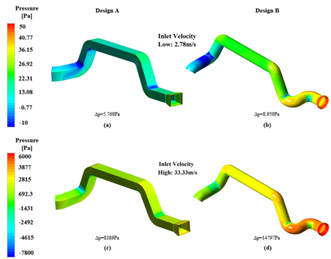
Figure 8 shows the pressure conditions to which both duct designs are subjected, corresponding to $2.78 \mathrm{~m} / \mathrm{s}$ and 33.33 $\mathrm{m} / \mathrm{s}$, respectively. At $2.78 \mathrm{~m} / \mathrm{s}$, Design A changes from $p_{{inlet}}=$ 2.594 Pa to $p_{{outlet}}=-3.175 \mathrm{~Pa}$, yielding an inlet-outlet drop of $\Delta \mathrm{p}=5.769 \mathrm{~Pa}$. Under the same conditions, Design B changes from $p_{{inlet}}=4.698 \mathrm{~Pa}$ to $p_{{outlet}}=-4.261 \mathrm{~Pa}$, with $\Delta \mathrm{p}=8.959 \mathrm{~Pa}$. Therefore, compared to $\mathrm{B}, \mathrm{A}$ shows a $44.8 \%$ lower inlet pressure, a 25.5% smaller outlet pressure magnitude $(\mathrm{p})$ , and a 35.6% lower overall drop.
At $33.33 \mathrm{~m} / \mathrm{s}$, Design A changes from $p_{\text {inlet }}=3180 \mathrm{~Pa}$ to $p_{\text {outlet }}=-5209 \mathrm{~Pa} (\Delta \mathrm{p}=8389 \mathrm{~Pa})$, while Design B changes from $p_{\text {inlet }}=6427 \mathrm{~Pa}$ to $p_{\text {outlet }}=-8370 \mathrm{~Pa} (\Delta \mathrm{p}=14797 \mathrm{~Pa})$. In this regime, A maintains a $50.5 \%$ lower inlet pressure, a $37.8 \%$ smaller outlet pressure magnitude, and a $43.3 \%$ lower inlet-outlet drop compared to B.
Figure 7. Air velocity distribution in ducts. At 2.78 m/s (a) Design A, (b) Design B. At 33.33 m/s (c) Design A, (d) Design B
Figure 8. Pressure Drop Distribution. At 2.78 m/s (a) Design A, (b) Design B. At 33.33 m/s (c) Design A, (d) Design B
At both speeds, the maximum pressure value is concentrated at the duct inlet, consistent with the flow stagnation effect at the entry lip. From this point onward, the pressure progressively decreases due to frictional losses and local accelerations induced by geometric changes. Model A maintains a more uniform distribution, reducing the magnitude of overpressures and depressions, whereas Model B presents more localized zones with sharp peaks and drops, associated with greater geometric complexity. These differences suggest that, for the evaluated conditions, A delivers a more efficient and predictable aerodynamic performance, while B requires more careful control of its geometric features to mitigate the observed losses and gradients.
The location of the extremes is explained by three well-known mechanisms:
(i) Stagnation at the inlet lip, where the flow decelerates locally, converting kinetic energy into static pressure and generating the p peak.
(ii) Cumulative pressure losses due to wall friction and geometric features (bends, transitions, and potential separations), which cause a progressive pressure decrease along the duct in accordance with Bernoulli’s principle with losses.
(iii) Discharge condition: upon exiting to the ambient, the jet undergoes acceleration; consequently, the immediate static pressure at the outlet can become low or even negative (gauge) relative to the reference. This effect is accentuated when contractions are present or when alignment is poor.
At higher velocities, all these mechanisms are amplified, explaining the more pronounced differences observed at 33.33 m/s.
3.3 Justification for the selection of the optimal design
The comparative analysis of velocity distribution and pressure drop justifies the selection of Design A for the subsequent stages of this research. Although Design B showed a higher outlet velocity at high speed, this advantage was offset by a substantially greater pressure drop (35.6% at low speed and 43.3% at high speed), mainly attributable to its geometric complexity and circular profile.
In contrast, Design A, with its rectangular profile, demonstrated a more efficient and reliable aerodynamic performance, characterized by significantly lower pressure losses. Such efficiency provides a more uniform and consistent airflow directed toward the engine, thereby offering improved conditions for long-term thermal management. Therefore, Design A has been selected as the optimal configuration for the detailed coupled heat transfer and airflow simulation including the engine.
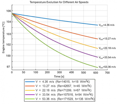
The results of the thermal analysis, summarized in Figure 9, reveal a direct relationship between the airflow outlet velocity and its cooling effectiveness. The analysis, which considered velocities from 4.36 m/s to 53.36 m/s, showed that increasing velocity leads to a higher Reynolds number (14,015.5 to 171,529.1), which in turn increases the Nusselt number (42.8 to 317.1) and the convective coefficient h (18.3 to 135.9 W/m²·K). This intensification of forced convection produced in a corresponding increase in the convective heat flow Q<sub>conv</sub> (from 4.16 W to 23.88 W).
This improved heat exchange led to a temperature drop (ΔT) in the engine's contour ranging from 1.11℃ to 7.22℃, with the most significant cooling occurring at higher velocities. However, the relationship between velocity and temperature reduction was not perfectly proportional, indicating that other factors, such as thermal resistances, natural convection, and radiation losses, also influenced the net cooling effect. The temperature curves showed a faster initial drop at higher velocities, but all conditions eventually stabilized as the system approached a dynamic equilibrium between the internal heat source and total heat losses.
It is important to note that, although the proposed ducts are described as implementable without major modifications, this statement requires qualification. From a geometric perspective, the ducts make use of the free space behind the fog lights, which minimizes interference with existing components. However, in practice, several issues must be considered to ensure real-world applicability. First, serviceability is critical, since the ducts could restrict access to nearby parts such as the radiator or suspension arms during maintenance. Second, integration with bodywork and underhood structures may demand minor adjustments or reinforcements to prevent contact under dynamic vibration. Third, production and installation costs should be carefully evaluated, as the chosen manufacturing process (e.g., injection molding or composite layup) and the assembly procedure can affect large-scale feasibility. For these reasons, while the design demonstrates aerodynamic and thermal advantages in the virtual domain, further work is required to fully validate its plug-and-play potential in commercial vehicles. In addition, future experimental validation under controlled operating conditions is essential to verify durability and long-term performance. Consideration of material fatigue and thermal cycling will also provide a clearer view of lifecycle reliability. These aspects, combined with real-world testing, will strengthen the transition from numerical modeling to industrial application.
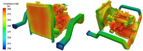
Figure 10 shows that, from an applied perspective, the results confirm the air jet effectively supplements the main cooling system, with its maximum impact occurring in the medium-to-high velocity range. The recorded maximum reduction of 7.22℃ should be evaluated within the context of the engine’s actual thermal load and operational conditions, as its overall contribution depends on factors such as flow geometry, effective impact area, and the capacity of the primary cooling system.
Figure 9. Engine temperature drop as a function of flow velocity
Figure 10. Integrated thermal model of the engine with model A duct for heat transfer analysis
At 120 km/h (33.33 m/s), the analytical results from MATLAB indicated an increase in the convective coefficient to h = 135.9 W/m²·K, which correlated with an engine temperature reduction of ΔT = 7.22℃ (from ~105℃ to ~97.78℃). The CFX simulation corroborated this finding by showing cooler isotherms in the areas of the engine impacted by the air jet from the ducts, which visually demonstrates a localized increase in heat transfer. The strong agreement between the analytical model and the simulation results confirms that the ducts intensify heat extraction and justify the observed temperature reduction.
A modal analysis was performed to evaluate the dynamic response of the duct under two different support configurations.
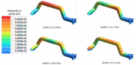
In the first configuration, the duct was constrained at the inlet and outlet (two supports). The first four natural frequencies were identified at 151.7 Hz, 223.2 Hz, 286.9 Hz, and 423.2 Hz, concentrating the highest effective modal masses in the Y (42.4%) and Z (40.9%) directions (Table 4). These modes were dominated by vertical bending and lateral-torsional deformations, mainly at the curved sections of the duct. Such behavior indicates potential susceptibility to vibration-induced fatigue if external excitation frequencies overlap with this range. The associated deformation patterns for the first four flexible modes are illustrated in Figure 11.
Table 4. Modal participation factors and effective mass for the first 20 flexible modes – two-support configuration
|
Flexible Mode |
Frequency (Hz) |
Modal Participation Factors 1° |
Effective Mass |
||||
|
X |
Y |
Z |
X (%) |
Y (%) |
Z (%) |
||
|
1 |
151.69 |
0.154 |
0.651 |
0.231 |
2.38 |
42.44 |
5.33 |
|
2 |
223.18 |
0.379 |
0.209 |
0.308 |
14.37 |
8.42 |
9.51 |
|
3 |
286.92 |
0.489 |
0.013 |
0.073 |
23.9 |
0.02 |
0.58 |
|
4 |
423.24 |
0.283 |
0.060 |
0.074 |
8.7 |
0.72 |
0.93 |
|
5 |
507.71 |
0.142 |
0.017 |
0.071 |
2.02 |
0.03 |
0.51 |
|
6 |
600.42 |
0.142 |
0.032 |
0.030 |
2.02 |
0.12 |
0.11 |
|
7 |
641.9 |
0.009 |
0.007 |
0.058 |
0.01 |
0 |
0 |
|
8 |
656.65 |
0.001 |
0.001 |
0.090 |
0.01 |
0 |
0 |
|
9 |
699.06 |
0.016 |
0.008 |
0.074 |
0.03 |
0.01 |
0.28 |
|
10 |
705.76 |
0.046 |
0.003 |
0.008 |
0.09 |
0 |
0 |
|
11 |
759.23 |
0.018 |
0.003 |
0.010 |
0.03 |
0 |
0.03 |
|
12 |
772.16 |
0.002 |
0.007 |
0.011 |
0 |
0 |
0 |
|
13 |
797.16 |
0.053 |
0.002 |
0.039 |
0.28 |
0 |
0.56 |
|
14 |
822.39 |
0.083 |
0.009 |
0.027 |
0.69 |
0.04 |
0.26 |
|
15 |
872.78 |
0.006 |
0.023 |
0.087 |
0 |
0 |
1.04 |
|
16 |
899.34 |
0.056 |
0.185 |
0.046 |
3.48 |
2.63 |
0.62 |
|
17 |
921.17 |
0.048 |
0.133 |
0.083 |
2.33 |
1.76 |
0.6 |
|
18 |
927.83 |
0.022 |
0.018 |
0.009 |
0.15 |
0 |
0.03 |
|
19 |
953.71 |
0.031 |
0.041 |
0.021 |
0.17 |
0.17 |
0.09 |
|
20 |
999.34 |
0.026 |
0.011 |
0.016 |
0.07 |
0.01 |
0.03 |
Table 5. Modal participation factors and effective mass for the first 20 flexible modes – three-support configuration
|
Flexible Mode |
Frequency (Hz) |
Modal Participation Factors 2° |
Effective Mass |
||||
|
X |
Y |
Z |
X (%) |
Y (%) |
Z (%) |
||
|
1 |
410.98 |
0.213 |
0.415 |
0.139 |
4.53 |
17.2 |
1.93 |
|
2 |
486.1 |
0.047 |
0.224 |
0.014 |
0.27 |
0.15 |
0.05 |
|
3 |
541.28 |
0.041 |
0.131 |
0.500 |
0.17 |
1.71 |
25 |
|
4 |
587 |
0.180 |
0.153 |
0.322 |
0 |
2.2 |
14.5 |
|
5 |
685.46 |
0.205 |
0.155 |
0.082 |
2.4 |
2.2 |
0.67 |
|
6 |
753.18 |
0.019 |
0.025 |
0.086 |
0.42 |
0.04 |
0.72 |
|
7 |
758.97 |
0.005 |
0.028 |
0.045 |
0 |
0.08 |
0.21 |
|
8 |
762.93 |
0.000 |
0.000 |
0.002 |
0 |
0 |
0 |
|
9 |
803.99 |
0.015 |
0.036 |
0.102 |
0.02 |
0.13 |
0.32 |
|
10 |
853.05 |
0.003 |
0.060 |
0.295 |
0 |
0.29 |
5.38 |
|
11 |
861.42 |
0.020 |
0.062 |
0.102 |
0 |
0 |
1.03 |
|
12 |
909.04 |
0.008 |
0.058 |
0.067 |
0 |
0.01 |
0.31 |
|
13 |
928.96 |
0.005 |
0.085 |
0.003 |
0 |
0 |
0 |
|
14 |
959.35 |
0.100 |
0.038 |
0.131 |
0.84 |
0 |
1.01 |
|
15 |
985.36 |
0.019 |
0.029 |
0.033 |
0.01 |
0.03 |
0.13 |
|
16 |
1027.8 |
0.044 |
0.038 |
0.054 |
0.27 |
0.01 |
0.19 |
|
17 |
1040.8 |
0.064 |
0.129 |
0.033 |
3.82 |
6.12 |
0.26 |
|
18 |
1055.2 |
0.057 |
0.195 |
0.046 |
3.23 |
3.79 |
0.13 |
|
19 |
1072.9 |
0.015 |
0.017 |
0.040 |
0 |
0 |
0.02 |
|
20 |
1078.3 |
0.016 |
0.009 |
0.085 |
0.03 |
0.01 |
0.72 |
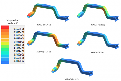
Figure 11. Potential deformation areas for the first five flexible modes of the duct – three-support configuration
Figure 12. Potential deformation areas for the first four flexible modes of the duct – two-support configuration
In the second configuration, a third support was added to the upper section of the duct to reduce the deformations observed in the previous case. This reinforcement significantly increased global stiffness: the first natural frequency rose from 151.7 Hz to 410.9 Hz, while subsequent modes appeared above 480 Hz. In addition, the effective modal mass in the Y direction, previously concentrated at 42.4%, was reduced to 17.2% in the first mode and remained below 2% in higher modes. Similarly, the Z-direction contributions did not exceed 25%. These results, summarized in Table 5, show that vibrational energy was redistributed toward higher frequencies and spread across multiple modes. The corresponding deformation patterns for the first five flexible modes are shown in Figure 12.
The study demonstrated that the redesigned rectangular duct (Design A) provides a more reliable and energy-efficient airflow delivery to the engine compartment. Beyond aerodynamic improvements, its implementation enhanced heat transfer by forced convection, achieving measurable reductions in surface temperature that complement the vehicle’s primary cooling system. Structural evaluations through modal analysis confirmed that the duct maintains adequate stiffness, and that the addition of an intermediate support further increases natural frequencies and reduces effective modal masses, minimizing the likelihood of resonance under operational excitations.
The methodological integration of analytical modeling in MATLAB with numerical simulations in ANSYS CFX ensured robust validation of the results, reinforcing confidence in the predictive capability of the proposed workflow. From a practical standpoint, the findings suggest that the solution can be extended to other vehicles facing similar challenges of thermal recirculation, with minimal structural modifications and without significant increases in computational or manufacturing cost.
Future work should include experimental validation under real operating conditions, evaluation of material durability under thermal–vibrational loads, and the integration of active cooling strategies to further enhance system performance. These aspects will provide a more comprehensive framework for the adoption of the proposed design in automotive applications.
We thank the Universidad Nacional de San Agustín de Arequipa for their support and knowledge, and NovaLabs for the resources and supervision provided.
|
$p $ |
static pressure, Pa |
|
$c_p$ |
specific heat at constant pressure, J·kg⁻¹·K⁻¹ |
|
$g_i$ |
gravity components, m·s⁻² |
|
$k$ |
turbulent kinetic energy, m²·s⁻² |
|
$h$ or $h_{ {convection }}$ |
convection coefficient, W·m⁻²·K⁻¹ |
|
$h_{{nat }}$ |
natural convection coefficient, W·m⁻²·K⁻¹ |
|
$q^{\prime \prime}$ |
imposed heat flux, W·m⁻² |
|
$q_{ {nat }}$ |
natural convection flux, W·m⁻² |
|
$q_{{convection }}$ |
net forced convection flux, W·m⁻² |
|
$m$ |
solid mass, kg |
|
Greek symbols |
|
|
$\rho$ |
density, kg·m⁻³ |
|
$\mu$ |
dynamic viscosity (laminar), Pa·s |
|
$\mu_t$ |
turbulent viscosity, Pa·s |
|
$\lambda$ |
thermal conductivity (laminar), W·m⁻¹·K⁻¹ |
|
$\lambda_t$ |
turbulent thermal conductivity, W·m⁻¹·K⁻¹ |
|
$\varepsilon$ |
turbulent dissipation rate, m²·s⁻³ |
|
$\sigma_k, \sigma_{\varepsilon}$ |
turbulent prandtl numbers for k, ε, – |
|
$C_\mu, C_{\varepsilon 1}, C_{\varepsilon 2}$ |
k–ε model constants, – |
|
$\mu_0$ |
viscosity at T0 (Sutherland), Pa·s |
|
$\sigma$ |
Stefan–Boltzmann constant, W·m⁻²·K⁻⁴ |
|
$\varepsilon\left(\frac{\varepsilon_f}{b}\right)$ |
emissivity (front/back), – |
|
Subscripts |
|
|
$x_i, x_j$ |
cartesian coordinates, m |
|
$u_i, u_j$ |
velocity components, m·s⁻¹ |
|
$T$ |
temperature, K |
|
$S_T$ |
source term in the energy equation, W·m⁻³ |
|
$P_K$ |
production of k, m²·s⁻³ |
|
$R$ |
gas constant (air), J·kg⁻¹·K⁻¹ |
|
$P$ |
thermodynamic pressure, Pa |
|
$T_0$ |
reference temperature (Sutherland), K |
|
$C$ |
sutherland constant, K |
|
$U$ |
average flow velocity, m·s⁻¹ |
|
$D\left(\right.$ or $\left.D_h\right)$ |
diameter (hydraulic), m |
|
$P r$ |
Prandtl number (cp .μ/k), – |
|
$R e$ |
Reynolds number (ρ.U.D/μ), – |
|
$T_W$ |
wall/surface temperature, K |
|
$T_{a m b}$ |
ambient temperature, K |
|
$\begin{aligned} & q_{\text {rad,front }}^{\prime \prime} \\ & q_{\text {rad,back }}^{\prime \prime}\end{aligned}$ |
radiative fluxes, W·m⁻² |
|
$A$ |
exchange area, m² |
|
$T$ |
time, s |
|
$Q$ |
energy extracted (qnet .t.A), J |
|
$\Delta T$ |
temperature reduction, K or ℃ |
|
$T_{{final }}$ |
estimated final temperature, K or ℃ |
|
$Nu$ |
Nusselt number (h.D/k), – |
[1] Song, X., Myers, J., Sarnia, S. (2014). Integrated low temperature cooling system development in turbo charged vehicle application. SAE International Journal of Passenger Cars-Mechanical Systems, 7(1): 163-173. https://doi.org/10.4271/2014-01-0638
[2] Patidar, A., Gupta, U., Marathe, N. (2013). Optimization of front end cooling module for commercial vehicle using CFD approach (No. 2013-26-0044). SAE Technical Paper. https://doi.org/10.4271/2013-26-0044
[3] Baskar, S., Doss, S.P.A. (2018). Investigation on underhood airflow management-effect of airflow statistics (No. 2018-28-0024). SAE Technical Paper. https://doi.org/10.4271/2018-28-0024
[4] Torregrosa, A., Galindo, J., Dolz, V., Royo-Pascual, L., Haller, R., Melis, J. (2016). Dynamic tests and adaptive control of a bottoming organic Rankine cycle of IC engine using swash-plate expander. Energy Conversion and Management, 126: 168-176. https://doi.org/10.1016/j.enconman.2016.07.078
[5] Song, X., Fortier, R., Sarnia, S. (2015). Underhood air duct design to improve A/C system performance by minimizing hot air recirculation. SAE International Journal of Passenger Cars-Mechanical Systems, 8(1): 338-345. https://doi.org/10.4271/2015-01-1689
[6] Larson, L., Woodiga, S. (2018). Aerodynamic investigation of cooling drag of a production pickup truck part 1: Test results. SAE International Journal of Passenger Cars-Mechanical Systems, 11(5): 477-491. https://doi.org/10.4271/2018-01-0740
[7] Zhao, L., Li, T., Guo, B., Wang, J., et al. (2023). Improving aero-thermal environment in vehicle under-hood through small modification upstream the cooling module. Proceedings of the Institution of Mechanical Engineers, Part D: Journal of Automobile Engineering, 237(5): 1003-1020. https://doi.org/10.1177/09544070221085967
[8] Franzke, R., Sebben, S., Willeson, E. (2022). Numerical investigation of the air flow in a simplified underhood environment. International Journal of Automotive Technology, 23(6): 1517-1527. https://doi.org/10.1007/s12239-022-0132-9
[9] Zhang, C., Uddin, M., Robinson, A.C., Foster, L. (2018). Full vehicle CFD investigations on the influence of front-end configuration on radiator performance and cooling drag. Applied Thermal Engineering, 130: 1328-1340. https://doi.org/10.1016/j.applthermaleng.2017.11.086
[10] Ferrari, C., Beccati, N., Pedrielli, F. (2023). CFD methodology for an underhood analysis towards the optimum fan position in a compact off-road machine. Energies, 16(11): 4369. https://doi.org/10.3390/en16114369
[11] Wang, Z., Wang, Y., Peng, C., Zheng, L. (2017). Experimental study of pressure back-propagation in a valveless air-breathing pulse detonation engine. Applied Thermal Engineering, 110: 62-69. https://doi.org/10.1016/j.applthermaleng.2016.08.144
[12] Corona Jr, J.J., Kaddoura, K.A., Kwarteng, A.A., Mesalhy, O., Chow, L.C., Leland, Q.H., Kizito, J.P. (2020). Comparison of two axial fans for cooling of electromechanical actuators at variable pressure. Thermal Science and Engineering Progress, 20: 100683. https://doi.org/10.1016/j.tsep.2020.100683
[13] Gong, C., Du, Y., Yu, Y., Chang, H., Luo, X., Tu, Z. (2022). Numerical and experimental investigation of enhanced heat transfer radiator through air deflection used in fuel cell vehicles. International Journal of Heat and Mass Transfer, 183: 122205. https://doi.org/10.1016/j.ijheatmasstransfer.2021.122205
[14] Tai, C.H., Cheng, C.G., Liao, C.Y. (2007). A practical and simplified airflow simulation to assess underhood cooling performance (No. 2007-01-1402). SAE Technical Paper. https://doi.org/10.4271/2007-01-1402
[15] Zarri, A., Botana, M.B., Christophe, J., Schram, C. (2024). Aerodynamic investigation of the turbulent flow past a louvered-fin-and-tube automotive heat exchanger. Experimental Thermal and Fluid Science, 155: 111182. https://doi.org/10.1016/j.expthermflusci.2024.111182
[16] Souby, M.M., Prabakaran, R., Liu, J., Kim, S.C. (2024). Heat transfer and power consumption of an optimized low-pressure compact drizzling cooling module integrated PEMFC stack radiator. International Communications in Heat and Mass Transfer, 159: 108046. https://doi.org/10.1016/j.icheatmasstransfer.2024.108046
[17] Datta, S.P., Das, P.K., Mukhopadhyay, S. (2014). Obstructed airflow through the condenser of an automotive air conditioner–Effects on the condenser and the overall performance of the system. Applied Thermal Engineering, 70(1): 925-934. https://doi.org/10.1016/j.applthermaleng.2014.05.066
[18] Toyota Motor Corporation. Manual de Reparación Toyota Hilux (modelo 2022). https://www.toyota-tech.eu.
[19] Vivarelli, G., Qin, N., Shahpar, S. (2025). A review of mesh adaptation technology applied to computational fluid dynamics. Fluids, 10(5): 129. https://doi.org/10.3390/fluids10050129
[20] Versteeg, H.K. (2007). An introduction to computational fluid dynamics the finite volume method, 2/E. Pearson Education India.
[21] Bergman, T.L. (2011). Fundamentals of Heat and Mass Transfer. John Wiley & Sons.
[22] Lukeman, Y., Lim, F.Y., Abdullah, S., R, Z., Shamsudeen, A., Khatim Hasan, M. (2012). Underhood fluid flow and thermal analysis for passenger vehicle. Applied Mechanics and Materials, 165: 150-154. https://doi.org/10.4028/www.scientific.net/AMM.165.150
[23] Kumar, C., Ademane, V., Madav, V. (2024). Experimental study of convective heat transfer distribution of non-interacting wall and perpendicular air jet impingement cooling on flat surface. Case Studies in Thermal Engineering, 60: 104532. https://doi.org/10.1016/j.csite.2024.104532
[24] Sekulic, D.P., Shah, R.K. (2023). Fundamentals of Heat Exchanger Design. John Wiley & Sons.
[25] Heat, F.O., Incropera, M.T.F.P. (2001). Fundamentals of Heat and Mass Transfer. Wiley India Pvt. Limited. https://books.google.com.pe/books/about/Fundamentals_Of_Heat_And_Mass_Transfer_5.html?id=ZHi6vzbt7gEC&redir_esc=y.
[26] Ulazia, A., Sáenz, J., Ibarra-Berastegi, G., González-Rojí, S.J., Carreno-Madinabeitia, S. (2019). Global estimations of wind energy potential considering seasonal air density changes. Energy, 187: 115938. https://doi.org/10.1016/j.energy.2019.115938
[27] Saito, Y., Mukai, K., Nakashima, S., Iwata, S., Shirota, M., Matsushita, Y. (2025). Effects of viscosity and shear-thinning characteristics of a liquid jet in air crossflow. International Journal of Multiphase Flow, 184: 105071. https://doi.org/10.1016/j.ijmultiphaseflow.2024.105071
[28] Finol, C.A., Robinson, K. (2006). Thermal modelling of modern engines: A review of empirical correlations to estimate the in-cylinder heat transfer coefficient. Proceedings of the Institution of Mechanical Engineers, Part D: Journal of Automobile Engineering, 220(12): 1765-1781. https://doi.org/10.1243/09544070JAUTO202
[29] Cengel, Y.A. (2006). Fluid Mechanics Fundamentals and Applications. McGraw Hill.
[30] White, F.M., Majdalani, J. (2006). Viscous Fluid Flow. pp. 433-434. New York: McGraw-Hill.
[31] Kornhauser, A.A., Smith, J.L. (1994). Application of a complex Nusselt number to heat transfer during compression and expansion. Journal of Heat Transfer, 116(3): 536-542. https://doi.org/10.1115/1.2910904
[32] Morel, T., Rackmil, C.I., Keribar, R., Jennings, M.J. (1988). Model for heat transfer and combustion in spark ignited engines and its comparison with experiments. SAE Transactions, 97(1988): 348-362.
[33] Batu, V. (2024). Fluid Mechanics and Hydraulics: Illustrative Worked Examples of Surface and Subsurface Flows. CRC Press.
[34] Reddy, J.N. (2015). An Introduction to Nonlinear Finite Element Analysis: With Applications to Heat Transfer, Fluid Mechanics, and Solid Mechanics. Oxford University Press.