Urban-Scale Building Air Change Rate Estimation Using Corrected Wind Speeds and Three-Zone Building Modeling

Figure 1 illustrates the workflow for deriving site and time-specific building ACRs in urban environments, which is tested by using the resulting ACRs as inputs to an hourly energy consumption model. First, z₀ is computed using UMEP for each wind direction, considering an amplitude of 30°. Second, z₀ is assigned to each building in the study area based on its location. Third, building-specific wind speed modifiers are calculated —accounting for location, orientation, and z₀ — to generate a database containing properties of all buildings to be analyzed. Finally, this database is used to generate CONTAM project files for each building and to run hourly ACR simulations using a user-defined weather file. Moreover, the accuracy of the proposed methodology is measured by comparing energy consumption models using the methodology presented by Mutani et al. [15] and three building ACR input scenarios: 1) fixed ACRs, 2) ACRs using the three-zone lumped-parameter model 3zLPM [10], and 3) using the building model of scenario 2 with UMEP-based real 3D urban environment wind speed correction presented in this paper. All three scenarios are compared with real measured hourly consumption data. The following subsections describe each of these steps in detail.

tu_pian_1.png

Figure 1. General methodology workflow

2.1 Aerodynamic Parameter Derivation with UMEP

The UMEP plugin requires several key inputs and settings to compute aerodynamic parameters (i.e., z₀) across the study area [6]:

• Analysis grid and search radius: A regular vector polygon grid defines the spatial resolution of the calculations. In this work, a 5 m by 5 m grid balances accuracy with computation time. A search radius of 200 m is used to aggregate surrounding morphometric parameters for each cell.
• Wind direction interval: In this work, a 30° wind direction interval is used. Smaller intervals would improve directional resolution but increase processing time.
• 3D built environment representation: Acceptable spatial resolution for the DSM and DEM is required, along with a raster of above-ground objects (obtained by subtracting the DEM from the DSM). While higher resolutions capture buildings and vegetation more accurately, but increase computational cost. In this work, a 1 m resolution is used for both DSM and DEM.
• Roughness calculation method: Among UMEP’s six options, Kanda’s empirical scheme is selected for dense urban contexts. It relates the calculation of z₀ to PAI, FAI, mean and maximum building heights, and building-height variability [5]. Using these inputs, UMEP computes z₀ for each grid cell and wind direction interval, forming the basis for subsequent steps in the workflow.

2.2 Building a database

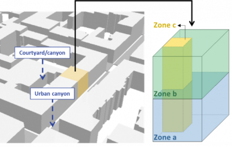
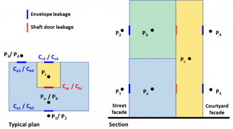
The three-zone model assumes each building as a part of a continuous urban canyon (Figure 2(a)); thus, this method is not applicable for detached buildings with four leakage sides. The representation of each single building (zones a, b, and c with leakage nodes 1-4) is illustrated in Figure 2(b). All geometric (volumes and node heights) and leakage parameters (leakage area of envelope and shaft doors) are derived from a polygon shapefile that contains each building’s height (Hbld) and construction period. Building footprint area is calculated in QGIS using a Field Calculator expression, e.g., $area, to populate an “Area” field. All other building related data are calculated using the main parameters (Hbld and construction period), as provided in Table 1.

2-1.png

(a)

2-2.png

(b)

Figure 2. Three-zone building simplification

3-1.png

3-2.png

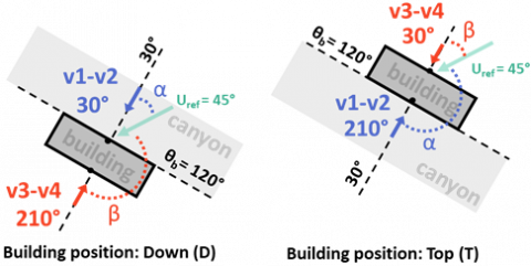
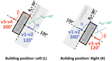
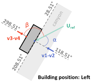
Figure 3. Building orientation (θ_b) and façade azimuth angle: canyon in blue, courtyard (or opposite) in red

Building orientation relative to the street network is determined by using QGIS’s Join by Nearest tool to link building centroids to the closest street segment. The streets can be derived either by using the open street map within QGIS or from other available regional databases [16]. By comparing the x,y coordinates of each building centroid (on the ground plane) to its joined street segment, buildings are classified as Top (T), Down (D), Left (L), or Right (R). This in turn establishes the wall-azimuth angles for both the canyon façade and the opposite courtyard façade (Figure 3). These orientations enable façade-specific wind-speed corrections in later steps (U_ref,corr).

Table 1 summarizes the required main building database for both wind speed modifier calculation and for CONTAM simulations.

Table 1. Calculated building parameters for wind speed correction and airflow modeling

For example, zone height (Ha, Hb) refers to the level height required by CONTAM, which is half the building height for zone a and zone b. The airflow element height (Hleakage) considered in the center of the zone levels (as illustrated previously in Figure 2). The shaft door multiplier is the number of doors per each link connecting zone a with c (through ac-ca) and zone b with c (through bc-cb) and is associated to the number of apartments per floor, which is then calculated based on the number of floors in the building. The typical leakage data (A_L) required for the envelope leakage calculations is mainly related to building construction period and building materials. In this work, a leakage area of 2.642 per unit area [cm²/m²] was used. Typical leakage data can be found in the study [17]. The total wall area, represented as an airflow element in Figure 2(b) (blue bold lines), is calculated using the geometrical attributes of the building calculated in earlier steps in QGIS.

With these building related data, each building record should contain all the fields required to generate façade-specific wind speed modifiers and to parameterize the three-zone airflow model for CONTAM.

2.3 Wind speed modifier calculations

Wind speed modifiers are required for CONTAM to correctly account for the wind pressure, which is significant driving force for air infiltration, on the analyzed façade points. Eq. (1) provides the wind pressure (P_w) calculated in CONTAM.

$P_w=\frac{\rho V_{m e t}^2}{2} C_h f(\theta)$         (1)

where,

ρ is the ambient air density [kg/m³];

V_met is the wind speed measured at meteorological station [m/s];

C_h is the wind speed modifier accounting for terrain and elevation effect;

$f(\theta)$ is the coefficient that is a function of the relative wind direction. referred to as the wind pressure profile.

From Eq. (1), the term $C_h f(\theta)$ links the wind direction to the façade azimuth angle (illustrated by the blue and red angles in Figure 3). CONTAM allows up to 16 angle/pressure coefficient pairs. These modifiers are calculated for each of the four façade points (1, 2, 3, and 4 in Figure 2(b)), across 30° wind direction intervals, ensuring that the directional variability of wind is accurately captured for each leakage point.

To derive these wind speed modifiers, the wind speed at each façade point is first corrected then it is used to obtain the modifier value for each point and angle. This process generates a set of wind speed modifiers for each building, tailored to its unique orientation and urban context. The following sections provide a detailed explanation of this calculation process.

2.3.1 Wind speed correction

Wind speed corrections are computed following the approach by Georgakis et al. [12, 13], which applies two models based on the reference wind speed (U_ref) from a weather station.

(1) When U_ref < 4 m/s [13]:

Using a simple linear correlation method (Eq. (2)):

$V_z=-0.537+0.957 z / w-0.012 \cdot \Delta T+0.0039 \cdot U_{\text {ref,corr }}$         (2)

where,

V_z is the corrected wind speed at height z [m/s];

z is the height of the analyzed point [m];

w is the width of the canyon or courtyard [m];

∆T is the temperature difference between the ambient air and the canyon (or building envelope) surface temperatures at height z can be calculated using: Eqs. (7), (8), and (9) [15].

U_ref,corr is the undisturbed wind speed corrected to account for the component perpendicular to the building façade [m/s], as illustrated previously in Figure 3.

(2) When U_ref ≥ 4 m/s [12]:

$V_{z, i}=U_{\text {ref,corr }} \cdot \log \left[\frac{z+z_0}{z_0}\right] / \log \left[\frac{z_{\text {ref }}+z_0}{z_0}\right]$          (3)

where,

z₀ is the roughness length derived from UMEP [m];

z_ref is the height of the reference weather station [m].

Thus, based on the hourly wind direction, the appropriate correction method is applied to compute wind speeds at points i = 1, 2, 3, and 4 (Figure 2).

2.3.2 Wind speed modifier

The modifiers M_z,i= (V_z,i / U_ref)² is calculated at each of the four points of each building for every hour.

2.3.3 Directional averaging

M_z,i is then averaged within 30° intervals of wind direction and used to define wind pressure coefficient profiles for the CONTAM models of each building [18]. At the end of this step, the building database will include, in addition to the parameters discussed in Section 2.2, data pairs describing four wind speed coefficient profiles for building openings P1 – P4, where each profile consists of 12 angles (0°, 30°, 60° … 330°) and modifier data points.

2.4 CONTAM input database and simulations

CONTAM simulates building airflow by solving a network of nodes (zones and duct junctions) connected by airflow paths (e.g., cracks, doorways, and duct segments) under the influence of driving forces — wind pressure, buoyancy (stack effect), and mechanical systems. To incorporate site specific wind effects, CONTAM requires as inputs:

• Weather File: A time series of outdoor parameters, i.e., ambient temperature [K], barometric pressure [Pa], wind speed [m/s], and wind direction [°]. The weather file should be compatible with CONTAM (.wth) [19].
• Building zones and airflow connections: A description of each zone (e.g., lower and upper living zones, shaft), including their volumes, temperatures, and interconnectivity. Interzone airflow is defined by mathematical relationships between airflow and pressure, referred to as CONTAM airflow elements, e.g., Leakage area and Large opening elements.
• Leakage Areas: this power law model in CONTAM can be based on data from building pressurization tests, which measure airflow rates across pressure differences.  For each flow coefficient (illustrated previously by blue and red bold lines in Figure 2), CONTAM requires the leakage area and test conditions, i.e., discharge coefficient (C_d), flow exponent (n), and reference pressure difference (∆P) [20]. Table 2 provides an example input data for Leakage Areas using the calculation method described by Usta et al. [14].

The complete building database generated in Section 2.3 serves as the base input for creating project files (.prj) for each analyzed building using CONTAM Factorial [21].

Table 2. Leakage area airflow element input in CONTAM

To enable batch simulation across an urban-scale building stock, a “flagged” project template was developed in combination with a Python script. This script reads the building database — including geometry, leakage parameters, and wind speed modifiers — and inserts the relevant values into the template to produce modified .prj files. The script then executes CONTAM simulations for all buildings in the directory and aggregates the resulting hourly building ACRs into a single spreadsheet, indexed by building ID.

This section presents the results obtained from each stage of the proposed methodology, beginning with the wind speed correction using UMEP, followed by the calculation of wind speed modifiers and the simulation of building-specific ACRs using the three-zone CONTAM model. Finally, the performance of the model is evaluated by comparing the resulting hourly ACR-based energy consumption estimates with real measured data under different ACR input scenarios.

4.1 UMEP results for wind speed modifier calculations

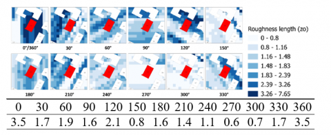
UMEP simulations generated building-specific values of z₀ for thirteen wind direction intervals at 30° intervals across the study area. Figure 5 presents an illustrative example of z₀ values assigned to a selected building for each wind direction interval: N = 0° or 360°, E = 90°, S = 180°, W = 270°. These direction-dependent z₀ values were then mapped to each hour of the meteorological time series, based on the prevailing wind direction.

5.png

Figure 5. Roughness length (z₀) maps for a sample building, with an average z₀ value assigned for each 30° wind direction

4.2 Wind speed correction and wind speed modifier acquisition

Following the methodology outlined in Section 2.1, hourly façade-level wind speeds were computed at the four points on each building’s façade (P1-P4 in Figure 2). These calculations account for building-specific urban geometry, including the relative position of each point with respect to the prevailing wind direction and its height above ground.

6-1.png

(a)

6-2.png

(b)

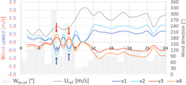
Figure 6. Hourly corrected wind speed at four façade points for a sample building, with the reference wind speed U_ref and direction W_dir,ref

Figure 6 presents an example of corrected hourly wind speeds for four façade points for a sample building. The graphs clearly highlight the influence of wind direction and point height on wind speed magnitude and sign. In particular, by comparing Figures 6(a) and 6(b), it can be observed that the wind speed at points 1 and 2, v1 and v2, (located on the street canyon façade and shown in blue) becomes negative — indicating leeward conditions — when the wind direction exceeds 208.51° or is below 28.5°. Furthermore, the reference wind speed (dotted line) shows significant reduction when the wind blows parallel to the canyon façade but remains relatively higher when the wind direction is close to perpendicular (between 110° and 130°).

This process ensures that each façade point is assigned a wind speed value that accurately reflects its height and orientation, capturing the directional asymmetry of wind exposure and enabling the model to distinguish effectively between windward and leeward conditions.

Using these corrected wind speeds, wind speed modifiers were then calculated using M_z,i = (Vz / Uref)².

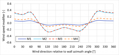
To align with CONTAM’s wind pressure input format, the hourly modifiers were averaged within each 30° wind direction interval (Figure 7) relative to the main façade (defined as 0°). In this profile, 0° represents wind blowing perpendicularly toward the façade, 90° indicates wind flowing parallel from the right, and 270° from the left; 180° is perpendicular away from the façade.

7.png

Figure 7. Wind speed coefficient profiles for four façade points as input for CONTAM

4.3 Hourly building ACR results

The hourly ACRs were calculated using the three-zone CONTAM model, incorporating the building-specific database developed in earlier steps. This database includes geometric properties, leakage parameters, and wind speed modifiers tailored to each building’s local urban context. The simulations were performed for all 27 buildings using CONTAM Factorial and the automated Python script for batch processing, achieving an elapsed simulation time of 13 seconds. This efficient workflow demonstrates the feasibility of applying the method to urban-scale analyses.

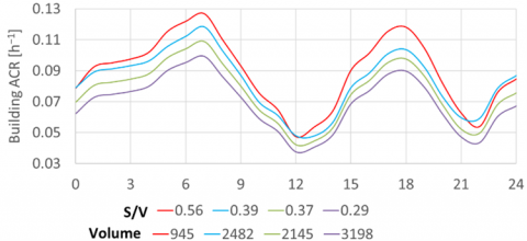
Figure 8 presents the hourly ACR profiles for four representative buildings, along with their respective volumes and surface-to-volume (S/V) ratios. The comparison reveals a consistent trend: buildings with higher S/V ratios resulted in higher ACRs. This is attributed to their relatively larger envelope area compared to the limited interior volumes. However, most residential buildings in Turin are compact with low S/V ratio, thus having low building ACRs [23].

The findings highlight the influence of building geometry on infiltration behavior, emphasizing the importance of volumetric scaling in airflow modeling. This geometric sensitivity further supports the application of the three-zone simplification used in this study, which has been previously validated against a detailed building model [14]. The comparison demonstrated that, despite the reduced level of detail, the simplified approach provides overall acceptable accuracy for buildings up to 16 floors (≈ 52 m) while improving computational efficiency.

8.png

Figure 8. Hourly building ACR for four selected buildings with their volume and S/V values

4.4 Hourly energy consumption results

The hourly ACRs generated in the previous step —simulated using the three-zone CONTAM model with wind speed modifiers derived from UMEP — were used as input for a process-driven, hourly energy consumption model [15]. Such urban scale energy models propose a promising approach also for the analyses of future expansion of district heating networks [24]. To assess the impact of this context-sensitive approach, the results of the energy consumption model using UMEP based ACRs were compared against two other ACR scenarios. The first scenario is using a fixed ACR based on the construction period of the building, the second scenario is ACR based on wind speeds corrected within the urban canyon via CFD simulations using a three-zone lumped parameter model (3zLPM) [10].

9.png

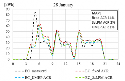
Figure 9. Hourly energy consumption (EC) using the three ACR scenarios and the measured data

All three scenarios were validated against measured hourly energy consumption data. Figure 9 illustrates the comparison of hourly energy consumption (EC) [kWh] for a representative day during the heating season using the three different ACR input scenarios. While the general trends in energy consumption are close, the daily Mean Absolute Percentage Error (MAPE) provided on the figure highlight the improvement in energy consumption calculations for both 3zLPM and UMEP ACR scenarios. Given inherent uncertainties in energy consumption measurement and modeling, daily-based MAPE and confidence interval (CI)—ranges around the monthly expected to contain the true value 95% of the time—provide realistic ranges on model performance. To better understand the results for the whole heating season, Tables 3 and 4 provide more pronounced differences.

Table 4 presents the MAPE for each scenario across representative months of the heating season, while Table 4 provides MAPE for selected days to provide more detailed insights. The results consistently show that dynamic ACR approaches—both UMEP-based and 3zLPM—outperform fixed ACR assumptions. Notably, the 3zLPM ACR scenario demonstrated slightly higher accuracy than UMEP ACR. This is likely due to the inclusion of CFD-derived adjustments in the 3zLPM, which better capture wind dynamics influenced by urban canyon geometry and façade irradiance effects. For February, the fixed-ACR MAPE is now 34.8% ± 8.5% (95% CI) vs. 20.4% ± 6.0% (95% CI), confirming a statistically significant improvement.

The daily MAPE results in Table 5 further highlight this trend, confirming that both dynamic ACR methods improve model performance, with 3zLPM offering a slight advantage in representing localized airflow effects more comprehensively.

Table 4. MAPE of monthly energy consumption estimates during the heating season for three ACR input scenarios

Table 5. Daily MAPE comparison of space heating demand predictions for selected days for three ACR input scenarios

Overall, the findings confirm that integrating dynamic, site-specific ACR values—reflecting each building’s unique urban context—substantially enhances the accuracy of simulated energy demand, reinforcing the value of this approach for detailed and context-aware urban energy modeling.