Layth H. Jawad![]()
© 2025 The author. This article is published by IIETA and is licensed under the CC BY 4.0 license (http://creativecommons.org/licenses/by/4.0/).
OPEN ACCESS
This paper presents a thorough numerical analysis of the thermal performance of vortex tube separators, comparing two designs: one with a complete cone valve and the other with a truncated cone valve. Using the RSM turbulence model in Ansys Fluent, the study investigates the effects of different design parameters and operating conditions on the efficiency of both models. The results show that increased intake pressure significantly improves thermal performance, with the complete cone valve model exhibiting a 122% increase in heat pump efficiency and a 57% increase in cooling capacity compared to the truncated cone model. Additionally, the study identifies optimal cold fraction values, which contribute to maximizing the vortex tube's performance. The simulations were validated through strong agreement with experimental data, confirming the model's reliability. The findings suggest that modifying the design, specifically by incorporating a complete cone valve, can significantly enhance the efficiency of vortex tube separators. These insights provide valuable guidance for improving vortex tube technology in practical applications such as thermal management systems, with potential benefits in various industrial settings.
numerical modeling, vortex separator, performance coefficient, gas turbulence
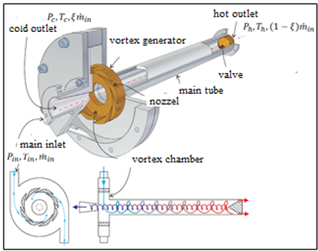
Thermal energy is managed nowadays by thermal devices such as heat exchangers, heat pumps, cooling machines, fins, phase change materials, and cyclone or vortex separators. Vortex separators are thermal-fluid devices that separate a compressed air stream, entering the device into two distinct streams: hot and cold. This separation occurs without any rotating parts or chemical reactions. The hot air exits through one outlet, while the cold air is expelled from another opposite the hot air outlet, as illustrated in Figure 1. This device was developed by the German scientist Hilsh in 1947 to benefit from this phenomenon in industrial applications, after which this device was called the Ranque-Hilsh vortex tube [1-4].
The vortex tubular separator consists of a chamber equipped with nozzles, the main tube, and a control valve, as shown in Figure 1. Compressed air enters the device through the vortex chamber, and the nozzles provide tangential movement within the device, forming two vortexes, one moving toward the hot outlet and the other toward the cold outlet. When the flow enters tangentially into the device, we have two vortices within the device that move in the opposite direction of each other. The first moves along the wall and forms a free, low-energy vortex; the other moves in the inner region and forms a forced, high-energy vortex. This flow structure is formed when the angular velocity of the flow increases towards the center to maintain a constant conservation of torque. As a result of this movement, the pressure near the wall becomes high, while the pressure decreases as we move towards the center of flow. This allows the air to expand from the place with high pressure at the wall to the place with low pressure at the center of the tube [5-8].
Figure 1. Components of vortex tube
This research aims to model the flow within a tubular separator to understand better the nature of the flow in these devices and the separation mechanism that divides the incoming air stream into two distinct streams: hot and cold. The goal is to develop this device further and enhance its efficiency by numerically comparing two models, ultimately improving its thermal performance. The significance of this research lies in its potential to increase the thermal efficiency of these devices, which have wide-ranging future applications, especially given their small size and low power requirements.
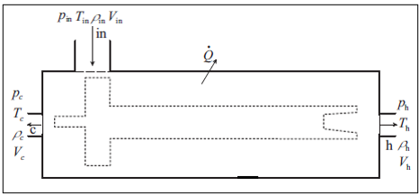
Thermodynamic analysis of the separator: Figure 2 shows the different areas within the vortex separation tube.
Figure 2. Conservation lows on vortex tube
Mass conservation equation: The mass entering the device per unit time equals the mass leaving it. This relationship is expressed mathematically during steady state as [9]:
$\dot{m}_{i n}=\dot{m}_c+\dot{m}_h$ (1)
where, $\dot{m}_{i n}$ is the mass flow entering the vortex chamber, $\dot{m}_c$ the flow leaving the cold outlet, and $\dot{m}_h$ the flow leaving the hot outlet [9].
The ratio $\xi=\frac{\dot{m}_c}{\dot{m}_{i n}}$ represents what is called the cold fraction, which represents the ratio of the time rate of the mass leaving the cold outlet concerning the time rate of the total mass entering the vortex chamber [10], and thus the equation becomes:
$\dot{m}_{i n}=\underbrace{(1-\zeta) \dot{m}_{i n}}_{\dot{m}_h}+\underbrace{\xi \dot{m}_{i n}}_{\dot{m}_c}$ (2)
Energy conservation equation: The total energy conservation equation for the vortex separator system, which does not perform any work and does not exchange heat with the surrounding environment in a steady state, can be expressed through the following relationship.
The term $h_o=\frac{1}{2} V^2+h$ represents the stagnation enthalpy or total enthalpy of the flow at the studied location. In contrast, h represents the static enthalpy of flow at the location or point studied. the subscribe (o) refers to the stagnation or total properties [11, 12].
Substituting $\xi=\frac{\dot{m}_c}{\dot{m}_{i n}}$ into the previous equation, we have:
$h_{o, i n}=\xi h \quad o, h_{o, c}$ (3)
But we have $h_o=c_p T_o$ , where $T_o$ represents the stagnation temperature or the total temperature, so we have:
$T_{o, i n}=\xi T_{o, c}+(1-\xi) T_{o, h}$ (4)
Hot temperature difference: It indicates the temperature difference between the hot outlet and the device inlet, represented by the relationship [13]:
$\Delta T_h=T_h-T_{i n}$ (5)
Cold temperature difference: It represents the static temperature difference between the device inlet and the cold outlet and is given by the relationship [13]:
$\Delta T_c=T_{i n}-T_c$ (6)
Vortex separator efficiency: The vortex separator works as a cooling machine and heat pump, which must be considered when studying the vortex separator. The performance factor of the vortex separator as a cooling machine is defined as the thermal cooling capacity $\dot{Q}_c$ with respect to the power expended on its operation and is given by the relationship [14]:
$\operatorname{COP}_c=\frac{\dot{Q}_c}{P}$ (7)
Refrigeration capacity $\dot{Q}_c$ is defined as the rate of heat withdrawn from the cooled gas from the inlet temperature to the cold outlet temperature and is given by the relationship [14]:
$\dot{Q}_c=\dot{m}_c c_p\left(T_{i n}-T_c\right)=\xi \dot{m}_{i n} c_p \Delta T_c$ (8)
P represents the power supplied to operate the compressor for the traditional refrigeration cycle. Still, there is no compressor in refrigeration systems using the vortex separator. The compressed air is supplied from a tank of air or compressed gas, so the power supplied to the separator is calculated as if it were a compressor compressing the gas by an isothermal process from the cold outlet pressure to the inlet temperature and pressure. Then the power supplied to the gas is [15]:
$P=\dot{m}_{i n} T_{i n} R \ln \left(\frac{P_{i n}}{P_c}\right)$ (9)
$\begin{gathered}C O P_c=\frac{\dot{Q}_c}{P}=\frac{\xi \dot{m}_{i n} c_p\left(T_{i n}-T_c\right)}{\dot{m}_{i n} R T_{i n} \ln \left(\frac{P_{i n}}{P_c}\right)}=\frac{\xi\left(T_{i n}-T_c\right)}{\alpha T_{i n} \ln \left(\frac{P_{i n}}{P_c}\right)} \\ =\frac{\xi \Delta T_c}{\alpha T_{i n} \ln \left(\frac{P_{i n}}{P_c}\right)}\end{gathered}$ (10)
When the machine operates as a heat pump, its performance is measured by the thermal power gained by the gas from the moment it enters until it exits through the hot outlet. This power is compared to the energy consumed during the compression process, which has been calculated previously [16].
$C O P_{h p}=\frac{\dot{Q}_{h p}}{P}$ (11)
Whereas $\dot{Q}_{h p}$ is the heat capacity acquired by the gas and given by:
$\dot{Q}_{h p}=\dot{m}_h c_p\left(T_h-T_{i n}\right)=(1-\xi) \dot{m}_{i n} c_p \Delta T_h$ (12)
Therefore, the coefficient of performance for the device as a heat pump is calculated according to the relationship [16]:
$\begin{array}{r}C O P_{h p}=\frac{\dot{Q}_{h p}}{P}=\frac{(1-\xi) \dot{m}_{i n} c_p\left(T_h-T_{i n}\right)}{\dot{m}_{i n} T_{i n} R \ln \left(\frac{P_{i n}}{P_c}\right)} \\ =\frac{(1-\xi)\left(T_h-T_{i n}\right)}{\alpha T_{i n} \ln \left(\frac{P_{i n}}{P_c}\right)} \\ =\frac{(1-\xi) \Delta T_h}{\alpha T_{i n} \ln \left(\frac{P_{i n}}{P_c}\right)}\end{array}$ (13)
$P_c$ was chosen because it is the smallest pressure from which it is compressed [17].
Physical model: The physical model consists of differential equations that govern flow, focusing on the analysis of the flow field within the separator and the mechanisms of energy transfer involved [18].
Motion and energy equations: The movement of fluids is governed by four differential equations: The continuity equation and the Navier-Stokes equation.
Continuity equation: The continuity equation expresses the principle of conservation of mass and states that the time rate of change of the mass of the control volume over time interval is equal to the difference between the rate of mass entering and exiting it. The relationship mathematically formulates it:
$\frac{\partial \rho}{\partial t}+\frac{\partial(\rho u)}{\partial x}+\frac{\partial(\rho v)}{\partial y}+\frac{\partial(\rho w)}{\partial z}=0$ (14)
where, $\rho$ represents density. u, v, w and w components of the velocity in the x, y, and z directions, respectively. Or in its compact form:
$\frac{\partial \rho}{\partial t}+\vec{\nabla} \cdot(\rho \vec{V})=0$ (15)
The first term represents the time rate, while the second term represents the convective term [19, 20].
Momentum equations: Newton's second law states that when a fluid's momentum changes, a force is acting on it. These equations are given as follows:
Momentum equation on the x-axis:
$\begin{aligned} \rho\left(\frac{\partial u}{\partial t}+u \frac{\partial u}{\partial x}+v \frac{\partial u}{\partial y}\right. & \left.+w \frac{\partial u}{\partial z}\right) \\ & =-\frac{\partial p}{\partial x}+\rho g_x \\ & +\mu\left(\frac{\partial^2 u}{\partial x^2}+\frac{\partial^2 u}{\partial y^2}+\frac{\partial^2 u}{\partial z^2}\right)\end{aligned}$ (16)
Momentum equation on the y axis:
$\begin{aligned} \rho\left(\frac{\partial v}{\partial t}+u \frac{\partial v}{\partial x}+v \frac{\partial v}{\partial y}\right. & \left.+w \frac{\partial v}{\partial z}\right) \\ & =-\frac{\partial p}{\partial y}+\rho g_y \\ & +\mu\left(\frac{\partial^2 v}{\partial x^2}+\frac{\partial^2 v}{\partial y^2}+\frac{\partial^2 v}{\partial z^2}\right)\end{aligned}$ (17)
Momentum equation on the z-axis:
$\begin{aligned} \rho\left(\frac{\partial w}{\partial t}+u \frac{\partial w}{\partial x}+v\right. & \left.v \frac{\partial w}{\partial y}+w \frac{\partial w}{\partial z}\right) \\ & =-\frac{\partial p}{\partial z}+\rho g_z \\ & +\mu\left(\frac{\partial^2 w}{\partial x^2}+\frac{\partial^2 w}{\partial y^2}+\frac{\partial^2 w}{\partial z^2}\right)\end{aligned}$ (18)
where, P represents pressure, g represents the acceleration of gravity, and $\mu$ represents viscosity, and is given according to the viscous heating model according to the Sutherland relationship [21]. This law results from the kinetic theory of gases using the forces inherent between molecules and relates viscosity changes to temperature changes and is given for two parameters by:
$\mu=\frac{c_1 T^{3 / 2}}{T+c_2}$ (19)
where, v represents the kinematic viscosity (Pa. s). T is the static temperature K. $c_1, c_2$ represents the coefficients of this law. For air at moderate pressure and temperature, the values of these coefficients are $c_1=1.458 \times 10^{-6} \frac{\mathrm{Kg}}{\mathrm{m} . \mathrm{s} . \mathrm{k}^{1 / 2}}$ and $c_2=110.4 K$ [22].
Energy conservation equation:
$\underbrace{\frac{\partial(\rho e)}{\partial t}}_1+\underbrace{\vec{\nabla}\left(\rho \vec{V} h_o\right)}_2=\underbrace{\vec{\nabla}(\vec{K} \vec{\nabla} T)}_3+\underbrace{\vec{\nabla}(\tau \vec{V})}_4+\underbrace{\vec{F}_b \cdot \vec{V}}_5+\underbrace{\dot{Q}}_6$ (20)
$e$ expresses the internal energy and is given by:
$e=h-P / \rho+1 / 2 V^2$ (21)
h is system enthalpy. $h_o$ is total enthalpy or stagnation enthalpy. $\tau$ is the shear stress resulting from viscous forces and is given by the relationship [21].
$\tau=\mu\left[\vec{\nabla} \vec{V}+(\vec{\nabla} \vec{V})^T-\frac{2}{3}(\vec{\nabla} \vec{V}) \delta\right]$ (22)
The first term represents the rate of change of the mass's energy over time. The second term accounts for the energy transported to and from the system by the movement of the fluid flow. The third term indicates the energy transferred into the system through conduction. The fourth term represents the energy dissipated within the bulk due to viscous forces. The fifth term reflects the power exchanged between the system and external volumetric forces acting upon it. Lastly, the sixth term describes the heat generated within the system due to an internal heat source [21].
Ideal gas law: The ideal gas law relating the state variables to the value of density changes as a function of absolute pressure and absolute temperature and given by $\rho=P_{a b} / R T$ [22].
Turbulence equations: Turbulence is defined as a random and chaotic fluctuation movement of molecules, where the speed and pressure components at any point in the flow suffer continuous changes over time. The cause of this turbulence is attributed to a source of change in the face of the flow that leads to the formation of a turbulent signal transmitted throughout the entire flow. The flow is classified into: Turbulent and laminar according to the Reynolds number criterion ($R e=\rho V L / \mu$), where L is a characteristic length and V is a characteristic velocity. In most cases, the flow can be classified as turbulent at a high Reynolds number, and at relatively low Reynolds numbers, the flow is classified as laminar [21].
The turbulence equations contain six additional unknowns and therefore need six additional equations or need turbulence models that reduce the number of equations.
Reynolds Stress Model (RSM): This model is based on solving seven equations which give the value of Reynolds stresses, and it is considered one of the types that simulate flows with complex strain fields or with clear physical forces, these equations in tensor form are [21]:
$\frac{D R_{i j}}{D t}=\frac{\partial R_{i j}}{\partial t}+C_{i j}=P_{i j}+D_{i j}-\varepsilon_{i j}+\Pi_{i j}+\Omega_{i j}$ (23)
where, $R_{i j}=\overline{u_i^{\prime} u_j^{\prime}}$ are Reynolds stresses. $C_{i j}=\frac{\partial}{\partial x_k}\left(\rho \bar{u}_k \overline{u_i^{\prime} u_j^{\prime}}\right)$ are R transmission by convection. $P_{i j}=-\left(R_{i m} \frac{\partial \bar{u}_j}{\partial x_m}+R_{j m} \frac{\partial \bar{u}_i}{\partial x_m}\right)$ are the rate of production of R. $D_{i j}=\frac{\partial}{\partial x_m}\left(\frac{\nu_t}{\sigma_k} \frac{\partial R_{i j}}{\partial x_m}\right)$ Transmission of R by diffusion. $\Pi_{i j}=-C_1 \frac{\varepsilon}{k}\left(R_{i j}-\frac{2}{3} k \delta_{i j}\right)-C_2\left(P_{i j}-\frac{2}{3} P \delta_{i j}\right)$ rate of transmission of R due to the mutual effect of stress and strain. $\Omega_{i j}=-2 \omega_k\left(\overline{u_j^{\prime} u_m^{\prime}} e_{i k m}+\overline{u_i^{\prime} u_m^{\prime}} e_{j k m}\right)$ rate of transmission R due to rotation. Here, K is the turbulence energy calculated from the relationship:
$k=\frac{1}{2}\left(\overline{u_1^{\prime 2}}+\overline{u_2^{\prime 2}}+\overline{u_3^{\prime 2}}\right)=\frac{1}{2}\left(R_{11}+R_{22}+R_{33}\right)$ (24)
$\varepsilon$ is energy dissipation and the constant $C_1=1.8 \& C_2=0.6$.
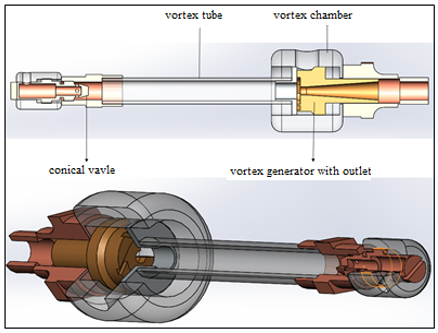
The vortex separator device utilized in this study comprises a vortex tube, vortex chamber, vortex generator, and cone valve, as illustrated in Figure 3.
Figure 3. Vortex tube cut view
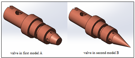
Figure 4. Studied model valves
Figure 4 shows the valve shape used in the considered models.
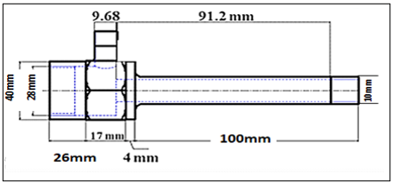
Figure 5 also shows the dimensions of the device used when the parts are assembled.
Figure 5. Vortex dimensions
Table 1 shows the air properties used in numerical modeling.
Table 1. Air property
|
Quantity |
Value |
Unit |
|
Density $\rho$ |
Ideal gas low |
Kg/m3 |
|
Heat capacity $c_p$ |
1006.43 |
J/Kg.K |
|
Viscosity $\mu$ |
Sutherland |
Pa.sec |
|
Molar Weight |
28.966 |
Kg/Kmol |
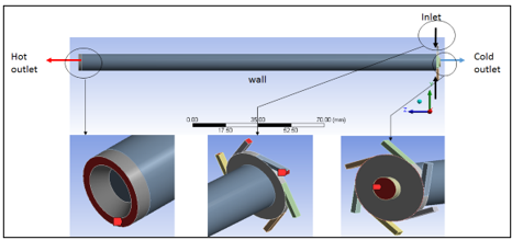
Table 2 and Figure 6 show the boundary conditions used in this modeling.
Table 2. Boundary conditions
|
Boundary Condition |
Surface |
Value |
|
Total pressure Inlet |
Inlet |
7 bar |
|
Total Temperature inlet |
301 K |
|
|
Static pressure outlet |
Hot outlet |
To archive specific cold fraction, vary 20-180 KPa |
|
Static pressure outlet |
Cold outlet |
20 KPa |
|
No slip condition |
Wall |
$v_x=0, v_y=0, v_z=0$ |
Figure 6. Boundary conditions
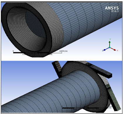
To address the mathematical model, the geometric model must be divided into a finite number of cells, known as the mesh. The differential equations that represent the geometric model will be solved on these cells. We used Ansys meshing software to generate the mesh, creating a pure hexahedral structural mesh to enhance computational accuracy and minimize the time required for the solution. Figure 7 illustrates the mesh that was utilized.
Figure 7. The mesh
Table 3 shows the characteristics and number of cells used in this model.
Table 3. Property of the mesh
|
Element Number |
701565 |
||
|
Node number |
760760 |
||
|
Aspect ratio |
Average |
max |
Min |
|
18.22 |
137 |
1.044 |
|
|
Orthogonal quality |
Average |
max |
Min |
|
0.88 |
1 |
0.1 |
|
To solve the main flow equations and to couple the velocity, pressure, and temperature, the program employs various algorithms to ensure that the solution converges effectively. The Coupled algorithm was selected in this research, as it solves the flow equations simultaneously. This approach allows for a faster convergence compared to the SIMPLE algorithm, which first calculates the pressure separately and then substitutes this value into the remaining equations to determine the velocity field, density, and other variables. This may require a longer computation time. In addition to choosing the Coupled algorithm, the pseudo-transient option was adopted, which allows a pseudo-time step that introduces an unsteady flow effect that can accelerate convergence. The basic equations, continuity, momentum, and turbulence model were chosen algebraically in the second-order discretization, which gives good solution accuracy while saving computation time compared to the higher degrees. Regarding the convergence conditions, convergence was based on all values of the flow equations taken (i.e., the residual reaching a value less than a pre-specified limit, $10^{-4}$ for the continuity equation, $10^{-5}$ for the rest of the equations).
Grid independence tests were conducted to ensure the accuracy of the numerical results. The computational domain was discretized using a pure hexahedral structural mesh generated in Ansys Meshing software. The mesh was refined iteratively to balance computational efficiency and result accuracy.
Initially, three different grid sizes were used: a coarse grid, a medium grid, and a fine grid. The solution converged when the residuals for all flow equations fell below a specified threshold. The temperatures at the cold and hot outlets were chosen as the key performance indicators for the grid independence analysis.
The results showed that the difference in temperature values between the medium and fine grids was minimal (less than 1%), indicating that the medium grid was sufficiently refined for accurate results. Further refinement did not significantly affect the performance, confirming the solution's grid independence.
The final mesh used in the simulations had an element number of 701,565 and a node number of 760,760. Its orthogonal quality was 0.88, and its average aspect ratio was 18.22, considered optimal for ensuring both computational efficiency and solution accuracy.
To verify the accuracy of the RSM turbulence model, a quantitative comparison was made between the simulation results and available experimental data. The focus was on temperature and performance coefficient values at the hot and cold outlets. The simulation results showed a small error (e.g., 5% for Model A and 4% for Model B) compared to the experimental data, confirming the model's reliability.
The error analysis was performed using the Root Mean Square Error (RMSE) and Mean Absolute Error (MAE), with values indicating a good agreement between the simulated and experimental results (e.g., RMSE = 1.2℃, MAE = 0.9℃). These low error margins demonstrate the accuracy of the RSM model in predicting the performance of the vortex tube separators.
The results confirm that the RSM turbulence model is suitable for simulating the complex, turbulent flow in vortex tube separators, making it an appropriate choice for further optimization studies.
6.1 Model A truncated cone valve
Numerical results indicate that the temperatures of the hot outlet increase with the increase in the value of the cold fraction and with the rise in the value of the entry pressure into the device, while the temperatures of the cold part decrease with the increase in the entry pressure. It is noted that there is a minimum value for the temperature of the cold outlet at a specific value of the cold fraction, after which the temperatures begin to rise, as they appear in Figure 8.
Figure 8 compares the experimental values obtained from the research paper [6] with those obtained by numerical modeling using the RSM turbulence model. The results show agreement between the numerical modeling and experimental results, confirming the CFD results' validity.
Temperature change charts with cold fractions can be interpreted as follows: The temperature changes between the hot and cold outlets are influenced by a series of processes, the most significant of which is direct adiabatic expansion between the inlet and the cold outlet. As theoretical analysis indicates, this process leads to a decrease in temperature, particularly near the cold outlet.
Figure 8. Temperatures at the cold (right) and hot (left) outlets numerically and experimentally in Model A
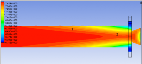
Figure 9. Constant entropy contour
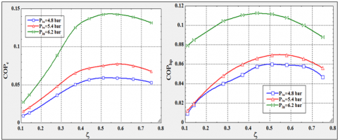
Figure 10. Coefficient of performance as cooling (left) and heating (right) machine in Model A
Furthermore, the drop in temperature observed in the center area results from heat exchange between the hot central region and the cooler peripheral area near the walls. Additionally, viscous heating, caused by friction, contributes to an increase in temperature, mainly due to irreversible processes within the device. As a result, the hot region continues to heat up due to the predominance of temperature increases linked to viscous heating. Figure 9 shows the numerical modeling results of the magnitude of constant $T / P^{\frac{k-1}{k}}$ contour, representing the adiabatic process along this line, which dominates near the cold outlet.
Figure 10 illustrates the device's performance coefficient when functioning as a refrigeration machine and a heat pump. From the figure, we can observe that there are optimal values for the cold fraction at which the performance coefficient reaches its maximum. Additionally, as the pressure of the gas entering the separator increases, the cold fraction required to achieve this optimal performance decreases.
Figure 11. Cold (right) and hot (left) outlet temperatures in the two models
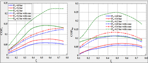
Figure 12. Coefficient of performance as cooling (left) and heating (right) machines in the two models
6.2 Model B full cone valve
In this part, we will compare the results of Model B to the results of the first Model A to compare the two models studied.
The numerical results obtained indicate that the behavior of the performance curves of the tubular separator with a complete cone valve is similar to the behavior of the performance curves of the tubular separator with a truncated cone valve in terms of improved performance with increasing inlet pressure and terms of the existence of optimal values for these curves at a specific cold fraction. However, a comparison of the performance between the separator in Model A and the separator in Model B indicates that the performance of the separator in Model B is better than the performance of the separator in Model A, as Figure 11 shows the hot and cold outlet temperature charts in Model B compared to these curves in Model A. We note that the hot outlet temperatures became higher in Model B compared to Model A, while the cold outlet temperature range became lower in Model B compared to Model A.
We observe that in Model B, the lowest temperature at the cold outlet occurs at a lower cold fraction compared to Model A. This phenomenon can be attributed to the complete cone design, which increases the pressure at hot and cold outlets. This increase in pressure reduces the speed of the axial flow of the return stream within the vortex chamber, thereby enhancing the mixing effectiveness. As a result, the optimum conditions begin to manifest at a lower cold fraction. Consequently, this leads to higher performance coefficients for the gas when using the full cone relative to the truncated cone, as illustrated in Figure 12.
We note that the optimal values occur at the highest inlet pressure value of 6.2 Bar. The performance coefficient of the device as a cooling machine increases in the second model by 57%. When the cold fraction in the second model is 18% higher than in the first model, the performance coefficient also increases as a heat pump in the second model by 122%, i.e., almost double what is in the first model at a cold fracture higher by 4%.
This study provides a comprehensive numerical investigation of the energy separation processes in vortex tube separators using two different valve designs: a truncated cone valve and a complete cone valve. The simulations were carried out using Ansys Fluent with the RSM turbulence model, which demonstrated strong agreement with experimental data, validating the accuracy of the simulation and the appropriateness of the turbulence model used.
The results revealed that increasing the inlet pressure significantly improved the thermal performance of both models. Additionally, the study identified optimal cold fraction values that maximize the separator’s thermal efficiency, which is crucial for optimizing the device's overall performance.
A key finding was that the vortex tube separator with a complete cone valve significantly outperforms the truncated cone valve model. Specifically, the full cone valve model exhibited a 57% improvement in the performance coefficient as a cooling machine and a remarkable 122% increase in performance as a heat pump. This improvement was observed when the cold fraction was 18% higher in the full cone valve model than the truncated cone model, with a 4% increase in cold fraction leading to nearly double the heat pump performance.
These findings highlight the potential for improving vortex tube separator designs by incorporating a complete cone valve to achieve higher efficiency. The results also provide valuable insights into optimizing thermal management systems, with practical implications for various industrial applications.
|
$\Delta T_h$ |
hot temperature difference, Kelvin (K) |
|
|
$\Delta T_c$ |
cold temperature difference, Kelvin (K) |
|
|
$\dot{Q}_c$ |
thermal cooling capacity, Watt (W) |
|
|
P |
power supplied to the gas, Watt (W) |
|
|
$C O P_c$ |
coefficient of performance, dimensionless |
|
|
$\dot{m}_{i n}$ |
mass flow entering, kg/s |
|
|
h |
enthalpy, J/kg |
|
|
T |
temperature, Kelvin (K) |
|
|
V |
velocity, m/s |
|
|
Re |
Reynolds number, dimensionless |
|
|
RSM |
Reynolds stress model |
|
|
Greek symbols |
||
|
$\xi$ |
cold fraction, dimensionless |
|
|
$\tau$ |
shear stress, N/m² |
|
|
$\rho$ |
density, kg/m³ |
|
|
$\mu$ |
dynamic viscosity, N·s/m² |
|
|
Subscripts |
||
|
h |
hot |
|
|
c |
cold |
|
|
in |
entering |
|
|
o |
stagnation |
|
[1] Shaji, K., Suryan, A., Kim, H.D. (2025). The effects of the vortex tube geometry on the thermal separation of compressible flow. Applied Thermal Engineering, 261: 125098. https://doi.org/10.1016/j.applthermaleng.2024.125098
[2] Meng, Z., Lin, S.R., Su, Z.Y., Ni, J., Wang, B.T., Zhu, Z.F., Liu, W.G. (2025). A coupled thermal mechanical hydrodynamic model for cutting of Ni-based superalloys cooled by a vortex tube. Journal of Manufacturing Processes, 137: 181–195. https://doi.org/10.1016/j.jmapro.2025.01.070
[3] Kuila, P.D., Melkote, S. (2020). Effect of minimum quantity lubrication and vortex tube cooling on laser-assisted micromilling of a difficult-to-cut steel. Proceedings of the Institution of Mechanical Engineers, Part B: Journal of Engineering Manufacture, 234(11): 1422–1432. https://doi.org/10.1177/0954405420911268
[4] Guo, Y.H., Chen, S.Q., Chen, F.X., Wu, S.X., Song, T.T., Wu, S.X., Zhu, Y.J. (2025). Vortex augmented heat and humidity energy extraction and the variation of vortex strength behind the string grid. Fuel, 387: 134297. https://doi.org/10.1016/j.fuel.2025.134297
[5] Haqqani, M.H., Azizuddin, M. (2024). A review on ranque-hilsch vortex tube and its usage in cooling system. Current Approaches in Engineering Research and Technology, 7: 31–50. https://doi.org/10.9734/bpi/caert/v7/1287
[6] Xue, Y.P., Binns, J.R., Arjomandi, M., Yan, H. (2019). Experimental investigation of the flow characteristics within a vortex tube with different configurations, Int. J. Heat Fluid Flow, 75: 195–208. https://doi.org/10.1016/j.ijheatfluidflow.2019.01.005
[7] Awan, O.A.A., Sager, R., Petersen, N.H., Wirsum, M., Juntasaro, E. (2025). Flow phenomena inside the Ranque-Hilsch vortex tube: A state-of-the-art review. Renewable and Sustainable Energy Reviews, 211: 115351. https://doi.org/10.1016/j.rser.2025.115351
[8] Alsaghir, A.M., Hamdan, M.O., Orhan, M.F. (2021). Evaluating velocity and temperature fields for Ranque-Hilsch vortex tube using numerical simulation. International Journal of Thermofluids, 10: 100074. https://doi.org/10.1016/j.ijft.2021.100074
[9] Sadeghiseraji, J., Moradicheghamahi, J., Sedaghatkish, A. (2021). Investigation of a vortex tube using three different RANS-based turbulence models. Journal of Thermal Analysis and Calorimetry, 143(6): 4039-4056. https://doi.org/10.1007/s10973-020-09368-6
[10] Bianco, V., Khait, A., Noskov, A., Alekhin, V. (2016). A comparison of the application of RSM and LES turbulence models in the numerical simulation of thermal and flow patterns in a double-circuit Ranque-Hilsch vortex tube. Applied Thermal Engineering, 106: 1244-1256. https://doi.org/10.1016/j.applthermaleng.2016.06.095
[11] Bagre, N., Parekh, A.D., Patel, V.K. (2022). Experimental and CFD analysis on the effect of various cold orifice diameters and inlet pressure of a vortex tube. Journal of Applied Fluid Mechanics, 16(1): 47-59. https://doi.org/10.47176/jafm.16.01.1271
[12] Hamdan, M.O., Al-Omari, S.A., Oweimer, A.S. (2018). Experimental study of vortex tube energy separation under different tube design. Experimental Thermal and Fluid Science, 91: 306-311. https://doi.org/10.1016/j.expthermflusci.2017.10.034
[13] Hu, Z.H., Li, R., Yang, X., Yang, M., Day, R., Wu, H.W. (2020). Energy separation for Ranque-Hilsch vortex tube: A short review. Thermal Science and Engineering Progress, 19: 100559. https://doi.org/10.1016/j.tsep.2020.100559
[14] Alsaghir, A.M., Hamdan, M.O., Orhan, M.F., Awad, M. (2022). Numerical and sensitivity analyses of various design parameters to maximize performance of a Vortex Tube. International Journal of Thermofluids, 13: 100133. https://doi.org/10.1016/j.ijft.2022.100133
[15] Parker, M.J., Straatman, A.G. (2021). Experimental study on the impact of pressure ratio on temperature drop in a Ranque-Hilsch vortex tube. Applied Thermal Engineering, 189: 116653. https://doi.org/10.1016/j.applthermaleng.2021.116653
[16] Cartlidge, J., Chowdhury, N., Povey, T. (2022). Performance characteristics of a divergent vortex tube. International Journal of Heat and Mass Transfer, 186: 122497. https://doi.org/10.1016/j.ijheatmasstransfer.2021.122497
[17] Koraim, E., Selim, S.M., Abdel-hamid, A.H.A., Hussien, A.A. (2023). Numerical investigation on the performance of vortex tube. Engineering Research Journal, 46(3): 323-338. https://doi.org/10.21608/erjm.2023.212195.1265
[18] Liang, F.C., Tang, G.X., Xu, C.Y., Wang, C., Wang, Z.Y., Wang, J.X., Li, N.M. (2021). Experimental investigation on improving the energy separation efficiency of vortex tube by optimizing the structure of vortex generator. Applied Thermal Engineering, 195: 117222. https://doi.org/10.1016/j.applthermaleng.2021.117222
[19] Zikanov, O. (2019). Essential Computational Fluid Dynamics. John Wiley & Sons.
[20] Tu, J., Yeoh, G.H., Liu, C., Tao, Y. (2023). Computational Fluid Dynamics: A Practical Approach. Elsevier.
[21] ANSYS Fluent documentation: Theory guide, 2016. (n.d.). https://dl.cfdexperts.net/cfd_resources/Ansys_Documentation/Fluent/Ansys_Fluent_Theory_Guide.pdf.
[22] ANSYS Fluent documentation: User guide, 2016. (n.d.). https://dl.cfdexperts.net/cfd_resources/Ansys_Documentation/Fluent/Ansys_Fluent_UDF_Manual.pdf.