Dayong Han![]() | Junhong Yang
| Junhong Yang![]() | Chao Guo
| Chao Guo![]() | Ping Liu
| Ping Liu![]() | Ce Gao
| Ce Gao![]() | Depeng Wang*
| Depeng Wang*![]()
© 2025 The authors. This article is published by IIETA and is licensed under the CC BY 4.0 license (http://creativecommons.org/licenses/by/4.0/).
OPEN ACCESS
With the continuous increase in global energy consumption, enhancing energy efficiency has become a crucial objective in the industrial sector. Mining equipment, as high-energy-consuming facilities, presents particularly significant challenges regarding energy consumption. Accurate energy consumption prediction for mining equipment is essential for improving energy utilization efficiency and reducing environmental impact. Traditional prediction methods often rely on empirical models or statistical regression analyses, which tend to yield large prediction errors when dealing with the complex operational processes and varying environmental factors associated with mining equipment. In recent years, deep learning techniques have been widely applied to energy consumption prediction in mining equipment, especially for multi-temporal scale forecasting. However, most methods fail to adequately consider thermodynamic processes, resulting in predictions that lack physical consistency. Existing studies predominantly focus on deep learning-based models, yet they struggle to effectively capture the intricate nonlinear relationships inherent in multi-temporal scale variations. Additionally, conventional models often neglect the significant impact of thermodynamic states on energy consumption, limiting their predictive accuracy. To address these challenges, this paper proposes a thermodynamically constrained artificial intelligence model for multi-temporal scale energy consumption prediction of mining equipment. Specifically, a bias-corrected spatiotemporal graph attention network is developed to adaptively capture energy consumption patterns across different temporal scales. Simultaneously, a thermodynamic constraint operator is incorporated to ensure the model adheres to thermodynamic principles, preventing physically inconsistent predictions. The proposed model offers a more accurate and scientifically grounded approach to optimizing energy efficiency in mining equipment.
mining equipment, energy consumption prediction, deep learning, spatiotemporal graph attention network, thermodynamic constraints, multi-temporal scale
With the continuous growth of global energy consumption, improving energy efficiency has become a core task across various industries, especially in the heavy industry sector [1-4]. As energy-intensive facilities [5], mining equipment has drawn increasing attention due to its energy consumption during operation [6, 7]. To achieve efficient energy utilization and reduce environmental impact, energy consumption prediction and optimization of mining equipment have become important research directions in mine management and energy management [8-10]. Accurate prediction of mining equipment energy consumption can help enterprises formulate reasonable production plans [11], optimize equipment scheduling [12], improve energy utilization efficiency [13], and reduce unnecessary energy waste. Traditional energy consumption prediction methods often rely on empirical models or statistical regression analysis, but these methods usually suffer from large prediction errors when facing complex equipment operation processes and variable environmental factors.
The energy consumption of mining equipment is influenced by multiple factors, including equipment operating conditions, environmental conditions, and time scales [14]. Deep learning methods for energy consumption prediction, especially for multi-temporal scale energy consumption prediction [15], can effectively capture complex nonlinear relationships and dynamic changes during equipment operation. However, existing deep learning models often overlook the impact of thermodynamic processes on energy consumption [16-18]. The importance of thermodynamic processes in mining equipment operation is self-evident, as the operational efficiency of the equipment is closely related to its internal thermodynamic state. Incorporating thermodynamic principles into deep learning models can significantly enhance the prediction accuracy and physical consistency of the models. Therefore, thermodynamically constrained artificial intelligence models have important research significance for multi-temporal scale energy consumption prediction of mining equipment.
Although some studies on mining equipment energy consumption prediction based on deep learning have been conducted, most of them remain at the level of traditional neural networks or regression models [19]. These methods perform poorly when handling multi-temporal scale problems, especially in terms of considering thermodynamic factors, due to the lack of effective constraint mechanisms. For example, although the method in the study of Li and Guo [20] can handle time series data, it fails to effectively capture energy consumption patterns over long temporal scales when facing complex variations across multiple time scales. Moreover, models without thermodynamic constraints are prone to generating prediction results that violate physical laws, which may lead to unreasonable optimization schemes in practical applications. Therefore, existing methods have considerable room for improvement in terms of model accuracy, physical consistency, and multi-temporal scale adaptability.
The main research content of this paper includes two parts. First, a multi-temporal scale energy consumption prediction model for mining equipment is constructed based on the bias-corrected spatiotemporal graph attention network. This model fully considers the energy consumption variations of mining equipment across different time scales and adaptively learns the energy consumption patterns through the spatiotemporal graph attention mechanism. Second, this paper introduces thermodynamic constraints and constructs a thermodynamic constraint operator in the energy consumption prediction model, ensuring that the model adheres to thermodynamic principles during the prediction process and avoids producing results that violate physical laws. This innovative approach not only improves the accuracy of mining equipment energy consumption prediction but also enhances the physical consistency and practicality of the model. Through these two aspects of research, the proposed model can provide a more accurate and scientific basis for optimizing the energy efficiency of mining equipment.
In the process of multi-temporal scale energy consumption prediction for mining equipment, the energy consumption demand of the equipment is usually influenced by multiple factors, including equipment operating conditions, environmental changes, and thermodynamic conditions. However, due to the complexity and variability of the equipment operation process, traditional energy consumption prediction models are susceptible to inherent bias, leading to prediction results deviating from the actual energy consumption demand and affecting energy efficiency optimization. Therefore, to address the inherent bias in the multi-temporal scale energy consumption prediction of mining equipment, this paper introduces the Bias-Corrected Spatiotemporal Graph Attention Network. By extracting temporal dependency features along the temporal dimension and integrating the state information of mining equipment along the spatial dimension, the network can more accurately capture the energy consumption variation patterns of the equipment at different temporal scales. On this basis, a bias tensor is constructed to model the inherent bias caused by the dynamic changes in equipment energy consumption demand, and bias correction is further performed by decoding the bias tensor information. Figure 1 shows the model structure.
Figure 1. Multi-temporal scale energy consumption prediction model structure for mining equipment
2.1 Spatiotemporal feature extraction encoding module
Figure 2 shows the schematic diagram of spatiotemporal feature extraction for mining equipment. In the spatiotemporal feature extraction encoding module of the network model, a graph embedding layer is introduced to effectively extract the features of the equipment in both temporal and spatial dimensions by constructing a spatiotemporal graph representation of mining equipment information. In the specific application scenario, the graph embedding layer first maps the state information of mining equipment to the graph structure, representing the positions and interaction relationships of mining equipment in the spatial dimension as a spatial graph HT={Ns, Rs}, while constructing a temporal graph HS={Nv, Rv} in the temporal dimension. The nodes in HT and HS are represented by Ns={nsv|v=1,2,...,SOBS} respectively, while the edges in HT and HS are represented by RS and Rv, respectively. Each node in the spatial graph represents the information of a piece of mining equipment, while the edges represent the interaction relationships between the equipment. These edges lack prior knowledge, so at the initial stage of the model, the weight values of the edges are assigned as 1 or 0, indicating whether there is an interaction between the mining equipment nodes. The temporal graph is constructed based on time series data, where each node represents the state information of the equipment at a specific time point, and the edges represent the interactions between equipment at different time points.
Figure 2. Schematic diagram of spatiotemporal feature extraction for mining equipment
In this way, the graph embedding layer effectively encodes mining equipment information into a graph structure in both temporal and spatial dimensions, facilitating the subsequent spatiotemporal graph attention mechanism to further learn spatiotemporal dependencies and thus improve the accuracy of energy consumption prediction. In the spatial graph, since there are usually strong interaction relationships between mining equipment information nodes, all interaction relationships between mining equipment information are assumed to be in a connected state during initialization, i.e., the elements in RS are assigned a value of 1. In the temporal graph, since the energy consumption of the equipment is influenced by its state before the current moment, the edges in the temporal graph are initialized as an upper triangular matrix, i.e., the elements in Rv are only allowed to connect forward to ensure that the model focuses only on past time information during learning, avoiding the introduction of future data influence. Specifically, initializing RS and Rv by assigning values of 1 or 0 is expressed as:
$R^s=\left[\begin{array}{cccc}1 & 1 & \cdots & 1 \\ 1 & 1 & \cdots & 1 \\ \vdots & \vdots & \cdots & \vdots \\ 1 & 1 & \cdots & 1\end{array}\right], R_v=\left[\begin{array}{cccc}1 & 1 & \cdots & 1 \\ 0 & 1 & \cdots & 1 \\ \vdots & \vdots & \cdots & \vdots \\ 0 & 0 & \cdots & 1\end{array}\right]$ (1)
The model further introduces a spatiotemporal feature extraction encoding module to capture the interaction characteristics of mining equipment in the temporal and spatial dimensions and effectively extract the relationships between mining equipment through the graph attention network. In this task, the key task is to calculate the interaction degree between mining equipment information points, i.e., the mutual correlation coefficient between nodes. By using the graph attention network, the model can calculate the interaction degree between mining equipment information nodes through the correlation between queries and keys, thereby effectively capturing the dependencies between mining equipment. The inner product result of queries and keys represents the correlation between mining equipment nodes and can reflect the mutual influence between equipment. For mining equipment energy consumption prediction, energy consumption demand is often influenced by equipment status and interactions. Therefore, through this mechanism, the network can automatically adjust the contribution of each node to the prediction result based on the interaction relationships between nodes.
Specifically, the first step of this module is to extract the interaction features of mining equipment information in the spatial dimension. In this step, traditional graph neural network methods may ignore the location information of the equipment. However, in the mining equipment energy consumption prediction task, the geographical location of the equipment has a significant impact on energy consumption relationships. Therefore, this study specifically embeds the location information into the mining equipment information graph, incorporating the spatial location information of mining equipment into the graph structure to ensure that the model fully considers the impact of location on mining equipment energy consumption. Assuming that the linear transformation function is represented by Linear(·), the location embedding information is represented by OT, and the weights of the linear transformation are represented by QOT, then we have:
$O_T=\operatorname{Linear}\left(Q_T^O, H_T\right)$ (2)
During the extraction of spatial dimension interaction features, the location embedding information first undergoes a linear transformation to generate queries and keys. This operation is a crucial step in the graph attention network. Through this linear transformation, the model can extract effective features from the mining equipment information and then use these features to capture the mutual influence between equipment in the spatial dimension. WT and JT respectively represent the queries and keys of each mining equipment in the spatial dimension, and these vectors help the model calculate the interaction weights between mining equipment in the subsequent steps. By using this approach, the model can not only identify the correlations between equipment in the spatial dimension but also dynamically adjust its importance in energy consumption prediction based on the location information of each piece of equipment. Assuming that the weights of the linear transformation are represented by QWT and QJT, the expressions for WT and JT are as follows:
$W_T=\operatorname{Linear}\left(Q_T^o, O_T\right)$ (3)
$J_T=\operatorname{Linear}\left(Q_T^J, O_T\right)$ (4)
Next, by performing an inner product calculation between queries WT and JT, the correlation or mutual correlation coefficient between mining equipment nodes can be obtained. To ensure that the calculated relationship coefficients conform to a standard probability distribution, they must be normalized using the Softmax function. The goal of this step is to convert the raw correlation coefficients obtained from calculations into attention weights, thereby generating the spatial adjacency matrix XT as shown in the following equation. This matrix reflects the interaction strength between equipment in the spatial dimension, helping the model effectively weight different equipment information in the subsequent processing. Assuming that the scaling factor is represented by (ft)1/2, we have the expression:
$X_T=\operatorname{softmax}\left(\frac{W_t J_t^S}{\sqrt{f_t}}\right)$ (5)
In addition to the extraction of interaction features in the spatial dimension, the core task of the spatiotemporal feature extraction encoding module also includes extracting the energy consumption dependency features of mining equipment information in the temporal dimension. Similar to the spatial dimension, the interaction features in the temporal dimension need to be extracted using the graph attention mechanism. The purpose of this process is to capture the energy consumption dependency relationships of equipment at different time points and convert them into a temporal adjacency matrix. In mining equipment energy consumption prediction, the energy consumption of the equipment is not only influenced by the current moment but also by the energy consumption of the equipment at the previous moment. Therefore, the temporal adjacency matrix reflects the energy consumption dependency of mining equipment in the time series, helping the model understand how equipment influences each other over consecutive time steps and providing more comprehensive sequential information for energy consumption prediction.
$O_S=\operatorname{Linear}\left(Q_S^o, H_S\right)$ (6)
$W_S=\operatorname{Linear}\left(Q_S^W, O_S\right)$ (7)
$J_S=\operatorname{Linear}\left(Q_S^J, O_S\right)$ (8)
$X_s^{\prime}=\operatorname{softmax}\left(\frac{W_S J_S^S}{\sqrt{f_S}}\right)$ (9)
After extracting temporal dimension features, the interaction between mining equipment information nodes is influenced by energy consumption correlation information at the current moment and previous moments. Therefore, to ensure the model adheres to this causality, when processing the temporal adjacency matrix, it is necessary to perform a pointwise multiplication operation between the temporal adjacency matrix and the adjacency matrix in the spatial graph, as shown in the following equation. This operation ensures that the model can only make predictions based on the past and current equipment energy consumption states, thus avoiding interference from future information on the current prediction.
$X_S=X_S^{\prime} \otimes R_v$ (10)
Finally, after processing through the graph attention network, the spatiotemporal feature extraction module obtains the spatial adjacency matrix XT and the temporal adjacency matrix XS, both containing interaction weight information. These two matrices represent the spatial interaction feature graph HT^={Ns, XT} and the temporal energy consumption dependency feature graph HS^={Nv, XS} of mining equipment, respectively. These two feature graphs integrate the interaction information of mining equipment in both temporal and spatial dimensions, providing sufficient spatiotemporal feature support for subsequent energy consumption prediction.
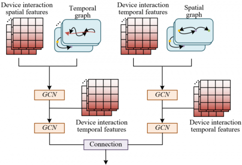
Figure 3. Processing procedure of the spatiotemporal feature fusion module
In mining equipment energy consumption prediction, the equipment’s state is not only affected by spatial location but also by the sequential associations and energy consumption patterns between equipment. To fuse the spatial interaction feature graph and the temporal energy consumption dependency feature graph extracted in the previous module, thereby obtaining more comprehensive spatiotemporal features, this study introduces a spatiotemporal feature fusion module. Figure 3 shows the processing procedure of the spatiotemporal feature fusion module. The key of the module lies in effectively aggregating the spatial interaction feature graph HT^ and the temporal energy consumption dependency feature graph HS^ of mining equipment through a graph convolutional network (GCN). Through this aggregation, the model can combine information from spatial and temporal dimensions, comprehensively reflecting the multi-level features of mining equipment, thereby providing more accurate input for subsequent energy consumption prediction. Assuming the nonlinear activation function is represented by δ(·), with PReLU function adopted here, and QT1, QS1, QT2, and QS2 representing the weights of the GCN, the formula for generating spatiotemporal fusion features is as follows:
$D_{T S}=\delta\left(X_S \delta\left(X_T N^s Q_{T 1}\right) Q_{S 1}\right)$ (11)
$D_{S T}=\delta\left(X_T \delta\left(X_S N_v Q_{S 2}\right) Q_{T 2}\right)$ (12)
$D=\operatorname{concat}\left(D_{T S}, D_{S T}\right)$ (13)
2.2 Bias correction decoding module
In the network model, the core task of the bias correction decoding module is to simulate and eliminate potential false associations in the training data through a bias tensor, thereby improving the prediction accuracy of the model. In mining equipment energy consumption prediction, real-world scenarios often involve numerous factors that change over time, such as vehicle stops or sudden increases in equipment information. These changes may lead to deviations between the training data and real-world scenarios. When there are more vehicle stops in certain scenarios in the training set, the model may mistakenly bind such bias information, which is unrelated to energy consumption, with the energy consumption association features of mining equipment, thereby affecting the prediction accuracy during the testing phase. To solve this problem, this study constructs a bias tensor z, combining it with spatiotemporal fusion features to simulate the bias information present in energy consumption demand. The shape of the bias tensor is identical to that of the spatiotemporal fusion features, and its function is to model potential false associations during the training process so that these biases can be eliminated in the subsequent correction process.
Figure 4. Structure diagram of the temporal convolutional network (TCN) used
In the bias correction module, the bias tensor and the spatiotemporal fusion features are input into the TCN for decoding. Figure 4 shows the structure diagram of the TCN used. Since the purpose of the bias tensor is to simulate bias information in energy consumption demand, the bias correction module subtracts the bias information from the decoded mining equipment energy consumption association information based on causal analysis, resulting in an output that more closely reflects actual energy consumption demand. To further enhance the model's adaptability and accuracy, the decoded bias information is processed through a learnable adaptive network layer, ensuring that the final output of the mining equipment energy consumption association prediction information can more accurately reflect the energy consumption variations of mining equipment across multiple time scales. Assuming the input and output of the TCN are represented by NIN and NOUT, and the number of TCN layers is represented by V, the calculation of the CN used in this study is as follows:
$N_{\text {OUT }}=\left[\operatorname{dropout}\left(O \operatorname{ReLU}\left(\operatorname{conv} 2 D\left(N_{I N}\right)\right)+N_{I N}\right)\right]_V$ (14)
In order to simulate and eliminate possible spurious correlations in the training data through the bias tensor, this study further sets up a bias correction decoding module to improve the model’s prediction accuracy. In the energy consumption prediction of mining equipment, real-world scenarios often include various dynamically changing factors, such as vehicle stops or sudden surges in device information. These changes may lead to deviations between the training data and the actual scenarios. When there are frequent vehicle stops in certain scenes of the training set, the model may mistakenly associate such bias information, which is unrelated to energy consumption, with the energy consumption correlation features of mining equipment, thereby affecting prediction accuracy during the testing phase. To address this issue, this study constructs a bias tensor, combining it with spatiotemporal fusion features to simulate the bias information present in energy consumption demands. In the bias correction module, the bias tensor and spatiotemporal fusion features are jointly input into the TCN for decoding. Since the role of the bias tensor is to simulate bias information in energy consumption demands, the bias correction module subtracts the bias information from the decoded mining equipment energy consumption correlation information based on causal analysis, obtaining an output that more closely approximates the true energy consumption demand. Figure 5 shows the causal convolution process. Assuming that the learnable adaptive network is represented by $\Theta$(·), the specific process is as follows:
$N_1=T C N(D)$ (15)
$N_2=T C N(C)$ (16)
$N=\Theta\left(N_1-N_2\right)$ (17)
Figure 5. Causal convolution process
In the scenario of multi-time-scale energy consumption prediction for mining equipment, changes in energy consumption are not only influenced by the operational status and modes of the equipment but also constrained by thermodynamic processes. When mining equipment is in operation, energy conversion and flow follow certain thermodynamic laws, such as the law of energy conservation and the second law of thermodynamics. Therefore, incorporating thermodynamic constraints into the mining equipment energy consumption prediction model can help the model more accurately capture the equipment's energy consumption patterns, ensuring that the model’s predicted energy consumption results comply with physical principles and avoiding abnormal predictions that violate thermodynamic laws. In this study, during the training process, a thermodynamic constraint operator is constructed to enable the model to continuously reference and learn physical characteristics related to thermodynamic laws in both the spatiotemporal feature fusion and prediction stages.
The introduced thermodynamic constraint operator aims to map the thermal efficiency curves and heat loss curves of mining equipment to multi-time-scale energy consumption data. Through this mapping relationship, the model ensures that the prediction process adheres to the thermodynamic laws in physics. Specifically, the thermal efficiency curve describes the energy conversion efficiency of the equipment under different operating states, while the heat loss curve represents the energy loss during the equipment's operation. By constructing the thermodynamic constraint operator, these physical characteristics can be mapped onto the specific energy consumption data, ensuring that the model's energy consumption prediction across multiple time scales reflects the actual physical behavior of the equipment. The construction principle of the thermodynamic constraint operator can be summarized in the following two steps: (1) Collect and analyze the thermal efficiency and heat loss data of mining equipment under different operating states to obtain the thermal efficiency curves and heat loss curves. These curves reflect the energy conversion and loss characteristics of the equipment under various operating conditions. (2) Associate these thermodynamic curves with specific energy consumption data to construct a mapping relationship, i.e., the thermodynamic constraint operator.
Before conducting the multi-time-scale energy consumption prediction experiments for mining equipment, this study first trains the thermodynamically constrained energy consumption prediction model neural network using pre-constructed thermodynamic data and minimizes the objective function below to train the model. Assuming that the thermal efficiency curve, heat loss curve, and temperature data of mining equipment are represented by qo, qF, and t, respectively, the constraint operator is represented by DΦ1, and the number of samples is denoted by V. This training process can be described by the following formulas:
$D_{\Phi_1}\left(q_o, q_F\right)=t$ (18)
${LOSS}_z\left(\Phi_1\right)=\frac{1}{V} \sum_{u=1}^V\left\|t_u-D_{\Phi_1}\left(q_o, q_F\right)\right\|_2^2$ (19)
Assuming that the conventional thermal efficiency curve and heat loss curve are represented by q, the prediction operator is represented by $D_{\Phi 2}$, and the original loss is represented by LOSSo($\Phi 2$), the multi-time-scale energy consumption prediction process and objective function of mining equipment before introducing the thermodynamically constrained neural network can be described as:
$D_{\Phi_2}(t, q)=q_o$ (20)
${LOSS}_o\left(\Phi_2\right)=\frac{1}{V} \sum_{u=1}^V\left\|q_{o_i}-D_{\Phi_2}(t, q)\right\|_2^2$ (21)
In the multi-time-scale energy consumption prediction process of mining equipment, the predicted values output by the prediction model are fed into the pre-trained thermodynamically constrained neural network model, and the constraint loss is obtained by calculating the error between the synthetic mining equipment energy consumption record and the actual mining equipment energy consumption record, as shown in the following formula:
${LOSS}_z\left(\Phi_1, \Phi_2\right)=\frac{1}{V} \sum_{u=1}^V\left\|t_u-D_{\Phi_1}\left(D_{\Phi_2}(t, q), q_F\right)\right\|_2^2$ (22)
Thus, the overall objective function of the prediction can be described as:
$\begin{gathered}{LOSS}_o\left(\Phi_1, \Phi_2\right)=\frac{\beta}{V} \sum_{u=1}^V\left\|q_{o_i}-D_{\Phi_2}(t, q)\right\|_2^2+\frac{\alpha}{V} \sum_{u=1}^V\left\|t_u-D_{\Phi_1}\left(D_{\Phi_2}(t, q), q_F\right)\right\|_2^2\end{gathered}$ (23)
Assuming that the influencing factors are represented by $\beta$ and $\alpha$, the simplified form is as follows:
${LOSS}_o\left(\Phi_1, \Phi_2\right)=\beta {LOSS}_o\left(\Phi_2\right)+\alpha {LOSS}_z\left(\Phi_1, \Phi_2\right)$ (24)
Figure 6 shows the multi-time-scale energy consumption prediction results of mining equipment using different methods under thermodynamic constraints, and Figure 7 presents the locally magnified comparison. From the data in the figures, it can be observed that the prediction results of the proposed method under thermodynamic constraints show a significant improvement in accuracy compared to other methods. Between sampling points 66 and 74, the predicted values of the proposed method are 9500, 9550, 9500, 10300, and 11300, which are relatively close to the actual measured values of 9500, 9400, 9750, 10750, and 11750. Particularly at sampling points 72 and 74, the predicted values of the proposed method exhibit smaller discrepancies from the actual measured values, whereas other methods such as SS-GAT and MM-GAT show larger prediction deviations at these points. After sampling point 74, the prediction values of the proposed method continue to maintain high accuracy, demonstrating stability and reliability across multiple time scales.
Figure 6. Multi-time-scale energy consumption prediction results of mining equipment using different methods under thermodynamic constraints
Figure 7. Locally magnified comparison of multi-time-scale energy consumption prediction results of mining equipment under thermodynamic constraints
From the data in Table 1, it can be seen that the proposed method shows lower error values in the energy consumption prediction results under thermodynamic constraints across multiple equipment categories, significantly improving prediction accuracy. For excavation equipment, transportation equipment, drainage equipment, ventilation equipment, loading equipment, and the integrated energy system, the Mean Absolute Error (MAE) of the proposed method is 0.63, 0.28, 0.36, 0.26, 0.23, and 0.35, respectively, while the Root Mean Square Error (RMSE) is 1.02, 0.44, 0.66, 0.47, 0.42, and 0.61, respectively. These results indicate that the proposed method outperforms other methods in most equipment categories, especially in transportation equipment and loading equipment, where its MAE and RMSE are significantly lower than those of other methods. For example, in transportation equipment, the MAE and RMSE of the proposed method are 0.28 and 0.44, significantly lower than SS-GAT's 0.48/0.86 and MM-GAT's 0.25/0.51.
Table 1. Comparison of multi-time-scale energy consumption prediction results of mining equipment using different methods under thermodynamic constraints
|
Algorithm/Dataset |
Experimental Results (MAE/RMSE) |
|||||
|
Excavation Equipment |
Excavation Equipment |
Drainage Equipment |
Ventilation Equipment |
Loading Equipment |
Integrated Energy System |
|
|
SS-GAT |
0.63/0.12 |
0.48/0.86 |
0.43/0.78 |
0.33/0.52 |
0.31/0.47 |
0.43/0.74 |
|
MM-GAT |
0.55/1.21 |
0.25/0.51 |
0.41/0.88 |
0.32/0.72 |
0.51/1.26 |
0.42/0.88 |
|
AGAT |
0.62/1.12 |
0.31/0.54 |
0.36/0.71 |
0.28/0.52 |
0.24/0.44 |
0.36/0.64 |
|
The Proposed Method |
0.63/1.02 |
0.28/0.44 |
0.36/0.66 |
0.26/0.47 |
0.23/0.42 |
0.35/0.61 |
Table 2. Ablation experiment results for determining the number of TCN layers in thermodynamic constraints
|
Number of Layers/Dataset |
Experimental Results (MAE/RMSE) |
|||||
|
Excavation Equipment |
Excavation Equipment |
Drainage Equipment |
Ventilation Equipment |
Loading Equipment |
Integrated Energy System |
|
|
1 |
0.66/1.12 |
0.31/0.57 |
0.37/0.67 |
0.26/0.47 |
0.25/0.44 |
0.37/0.67 |
|
2 |
0.62/1.12 |
0.28/0.45 |
0.36/0.66 |
0.26/0.47 |
0.23/0.42 |
0.35/0.61 |
|
3 |
0.72/1.16 |
0.28/0.51 |
0.38/0.75 |
0.27/0.51 |
0.23/0.41 |
0.37/0.68 |
|
4 |
0.67/1.17 |
0.47/0.42 |
0.37/0.72 |
0.26/0.47 |
0.23/0.42 |
0.43/0.65 |
|
5 |
0.81/1.36 |
0.36/0.51 |
0.38/0.74 |
0.27/0.48 |
0.24/0.42 |
0.42/0.72 |
According to the data in Table 2, the number of TCN layers significantly impacts the energy consumption prediction results under thermodynamic constraints. When the number of TCN layers is set to 2, the overall performance is optimal, especially in the prediction of the integrated energy system, where the MAE and RMSE are 0.35 and 0.61, respectively. Furthermore, in the energy consumption predictions for excavation equipment, transportation equipment, drainage equipment, ventilation equipment, and loading equipment, the MAE and RMSE with 2 TCN layers are also significantly lower than those with other layer numbers. Specifically, the MAE and RMSE for transportation equipment are 0.28 and 0.45, respectively, while those for loading equipment are 0.23 and 0.42. These results suggest that when the number of TCN layers is set to 2, the model captures the energy consumption patterns more accurately, thereby improving prediction precision.
Table 3. Ablation experiment results for determining bias tensors under thermodynamic constraints
|
Bias Tensor/Dataset |
Experimental Results (MAE/RMSE) |
|||||
|
Excavation Equipment |
Excavation Equipment |
Drainage Equipment |
Ventilation Equipment |
Loading Equipment |
Integrated Energy System |
|
|
Zero Tensor |
0.63/1.12 |
0.28/0.45 |
0.38/0.66 |
0.26/0.47 |
0.23/0.42 |
0.35/0.61 |
|
Random Tensor |
0.67/1.26 |
0.28/0.48 |
0.36/0.66 |
0.26/0.45 |
0.22/0.42 |
0.36/0.66 |
|
Average Tensor |
0.72/1.37 |
0.27/0.48 |
0.37/0.71 |
0.27/0.47 |
0.22/0.41 |
0.37/0.71 |
|
Baseline Model |
0.62/1.18 |
0.31/0.54 |
0.36/0.71 |
0.28/0.52 |
0.24/0.44 |
0.36/0.66 |
According to the data in Table 3, introducing different types of bias tensors under thermodynamic constraints has a significant impact on the performance of the energy consumption prediction model. When using the zero tensor as the bias tensor, the MAE and RMSE for the integrated energy system are 0.35 and 0.61, respectively, representing the best performance. In the predictions for excavation equipment and loading equipment, the MAE and RMSE with the zero tensor are 0.63/1.12 and 0.23/0.42, respectively, also demonstrating superior performance. In contrast, the introduction of random tensors and average tensors generally leads to higher errors. For example, the RMSE for random tensors in excavation equipment reaches 1.26, while the RMSE for average tensors in drainage equipment is 0.71. The baseline model exhibits relatively higher prediction errors in most equipment categories, although its performance in excavation equipment is comparatively better.
In this study, the experimental results shown in Figure 8 demonstrate that the proposed Adaptive Bias Correction Spatio-Temporal Graph Attention Network model performs excellently in predicting the energy consumption of mining equipment. Specifically, the model accurately captures the energy consumption variations of mining equipment across different time scales, with the regression line of the predicted results and actual measurements almost aligning with the diagonal line, indicating a high degree of agreement between predicted and actual values. Furthermore, from the distribution of predicted and actual measured values, the two distributions are relatively consistent, further validating the model's superiority in handling multi-time scale energy consumption prediction tasks. Further analysis reveals that although the regression line shows a slight deviation from the diagonal, the magnitude of this deviation is minimal and does not significantly affect the prediction accuracy. In contrast, traditional models under the same experimental conditions exhibit a noticeable deviation between the regression line of predicted results and measured values relative to the diagonal, with larger differences in the distribution of predicted and measured values. These results indicate that the proposed method not only achieves higher consistency and accuracy in predicting mining equipment energy consumption but also ensures the physical rationality and practicality of the prediction results by introducing thermodynamic constraints, significantly enhancing the overall performance of the prediction model.
Figure 8. Intersection and distribution of multi-time scale energy consumption prediction and measurement results for mining equipment under thermodynamic constraints
This study consists of two main parts: first, a multi-time scale energy consumption prediction model based on the Adaptive Bias Correction Spatio-Temporal Graph Attention Network was constructed. This model fully considered the energy consumption variations of mining equipment across different time scales and adaptively learnt the energy consumption patterns under different time scales through the spatio-temporal graph attention mechanism. Second, thermodynamic constraints were introduced by constructing a thermodynamic constraint operator within the energy consumption prediction model, ensuring that the model follows thermodynamic principles during the prediction process, thereby avoiding physically unreasonable prediction results.
Comprehensive experimental results show that the proposed model performs excellently in predicting mining equipment energy consumption, with prediction results highly consistent with actual measurements and good distribution consistency. Compared to traditional models, the proposed model not only improves the accuracy of energy consumption predictions but also enhances the physical rationality of the prediction results through thermodynamic constraints, demonstrating significant practical value. The limitations of this study lie in the fact that, although the model performs well on experimental data, more external disturbance factors and complex working conditions may need to be considered in practical applications. Future research directions may focus on enhancing the generalization capability and adaptability of the model while further optimizing the thermodynamic constraint mechanism to explore its effectiveness and practicality in broader application scenarios.
[1] Pérez-Lombard, L., Ortiz, J., Velázquez, D. (2013). Revisiting energy efficiency fundamentals. Energy Efficiency, 6: 239-254. https://doi.org/10.1007/s12053-012-9180-8
[2] Dlamini, T., Mwashita, W. (2023). Enhancing Energy Efficiency in IoT-WSN Systems via a Hybrid Crow Search and Firefly Algorithm. Journal of Sustainability for Energy, 2(4): 197-206. https://doi.org/10.56578/jse020403
[3] Liu, Y.L., Lin, K.Y. (2023). Enhancing energy efficiency in sow houses: An annual temperature regulation system employing heat recovery and Photovoltaic-Thermal Technology. Journal of Sustainability for energy, 2(2): 76-90. https://doi.org/10.56578/jse020204
[4] Patil, G., Tiwari, C., Kavitkar, S., Makwana, R., Mukhopadhyay, R., Aggarwal, S., Betala, N., Sood, R. (2025). Optimising energy efficiency in India: A sustainable energy transition through the adoption of district cooling systems in Pune. Challenges in Sustainability, 13(1): 1-17. https://doi.org/10.56578/cis130101
[5] Kumari, P., Mamidala, V., Chavali, K., Behl, A. (2024). The changing dynamics of crypto mining and environmental impact. International Review of Economics & Finance, 89: 940-953. https://doi.org/10.1016/j.iref.2023.08.004
[6] Sahoo, L.K., Bandyopadhyay, S., Banerjee, R. (2014). Benchmarking energy consumption for dump trucks in mines. Applied Energy, 113: 1382-1396. https://doi.org/10.1016/j.apenergy.2013.08.058
[7] Aramendia, E., Brockway, P.E., Taylor, P. G., Norman, J. (2023). Global energy consumption of the mineral mining industry: Exploring the historical perspective and future pathways to 2060. Global Environmental Change, 83: 102745. https://doi.org/10.1016/j.gloenvcha.2023.102745
[8] Attari, M.Y.N., Miandoab, T.F., Ejlali, B., Torkayesh, A.E. (2021). Fuel consumption in mining industry using partial least squares structural equation modeling approach. International Journal of Energy Sector Management, 15(6): 1122-1143. https://doi.org/10.1108/IJESM-07-2020-0020
[9] Fischer, S., Szürke, S.K. (2023). Detection process of energy loss in electric railway vehicles, Facta Universitatis, Series: Mechanical Engineering, 21(1): 81–99. https://doi.org/10.22190/FUME221104046F
[10] Bahadori, M., Mousavi, S.M. (2022). Investigation of the effects of rock dynamic hardness on the energy consumption in the crushing unit, case study: Midouk copper mine. Applied Earth Science, 131(4): 193-205. https://doi.org/10.1080/25726838.2022.2095149
[11] Lasla, N., Al-Sahan, L., Abdallah, M., Younis, M. (2022). Green-PoW: An energy-efficient blockchain Proof-of-Work consensus algorithm. Computer Networks, 214: 109118. https://doi.org/10.1016/j.comnet.2022.109118
[12] Soofastaei, A., Aminossadati, S.M., Arefi, M.M., Kizil, M.S. (2016). Development of a multi-layer perceptron artificial neural network model to determine haul trucks energy consumption. International Journal of Mining Science and Technology, 26(2): 285-293. https://doi.org/10.1016/j.ijmst.2015.12.015
[13] Singh, S., Yassine, A. (2017). Mining energy consumption behavior patterns for households in smart grid. IEEE Transactions on Emerging Topics in Computing, 7(3): 404-419. https://doi.org/10.1109/TETC.2017.2692098
[14] Cheskidov, V.I., Kortelev, O.B., Aleksandrov, A.N., Il’bul’din, D.K. (2004). Estimation criteria for energy consumption by mining equipment in quarries. Journal of Mining Science, 40(4): 380-383. https://doi.org/10.1007/s10913-004-0021-9
[15] Gabaldon, E., Lerida, J. L., Guirado, F., Planes, J. (2017). Blacklist muti-objective genetic algorithm for energy saving in heterogeneous environments. The Journal of Supercomputing, 73(1): 354-369. https://doi.org/10.1007/s11227-016-1866-9
[16] Stepanov, V.S., Stepanova, T.B. (2004). Energy demand forecasting by thermodynamic analysis of energy consumed processes. Energy Sources, 26(7): 647-660. https://doi.org/10.1080/00908310490445526
[17] Tsirlin, A.M., Balunov, A.I., Sukin, I.A. (2016). Estimates of energy consumption and selection of optimal distillation sequence for multicomponent distillation. Theoretical Foundations of Chemical Engineering, 50: 250-259. https://doi.org/10.1134/S0040579516030131
[18] Zambrana, D., Aranda, A., Ferreira, G., Barrio, F. (2012). Energy-flow methodology for thermodynamic analysis of manufacturing processes: A case study of welding processes. Defect and Diffusion Forum, 326: 366-371. https://doi.org/10.4028/www.scientific.net/DDF.326-328.366
[19] Kuo, C.F.J., Lin, C.H., Lee, M.H. (2018). Analyze the energy consumption characteristics and affecting factors of Taiwan's convenience stores-using the big data mining approach. Energy and Buildings, 168: 120-136. https://doi.org/10.1016/j.enbuild.2018.03.021
[20] Li, Y., Guo, S. (2022). Real time prediction method of energy consumption of geothermal system in public buildings based on wavelet neural network. Thermal Science, 26(3): 2373-2384. https://doi.org/10.2298/TSCI2203373L