Eugenie Geraldine Ngah Abena![]() | Donatien Njomo
| Donatien Njomo![]() | Daniel Roméo Kamta Legue*
| Daniel Roméo Kamta Legue*![]()
© 2024 The authors. This article is published by IIETA and is licensed under the CC BY 4.0 license (http://creativecommons.org/licenses/by/4.0/).
OPEN ACCESS
This study aims to analyse the influence of cementing and thermal insulation on the pressure-volume-temperature (PVT) behaviour of crude oil during production. The idea is to identify the key parameters that have an impact on the PVT behaviour and to develop a model that accurately predicts the PVT behaviour of crude oil in offshore horizontal wells. The methods used will include numerical simulations and analysis of field data from well EKM-032 in the RIO DEL REY region of Cameroon. The results, taking into account the various intrinsic parameters, will provide a complete understanding of the PVT behaviour of crude oil in offshore horizontal wells and the development of a predictive model that can be used to optimise crude oil production.
cementation, thermal isolation, offshore, horizontal well and EKM-032
Offshore exploitation of oil deposits presents a major challenge, characterized by extreme environmental conditions and depths that are increasingly difficult to access [1]. The use of innovative horizontal well technology is currently one of the realistic and effective solutions in a context of declining production and fluctuating hydrocarbon prices due to their improved capacity compared to vertical wells [2, 3]. Due to marine conditions, inadequate heat transfer can cause variations in the PVT properties of oil during production; this can cause problems such as the crystallization of paraffins, which can block the pores of the reservoir and reduce permeability [4]. Pressure drops along the well can be aggravated by inadequate heat transfer. These pressure drops, combined with fluctuating temperatures, create an environment conducive to the formation of paraffins. These wax deposits can act as plugs, leading to flow problems, reduced production and increased operational costs [5].
The production rate being intrinsically linked to the stability of the PVT properties. Inappropriate temperature variations inevitably lead to variations in oil viscosity and density, directly affecting flow rate. Effective thermal insulation becomes crucial to maintain stable production conditions, thereby optimizing the yield of the offshore well [6]. The first models for interpreting temperature variations in oil wells were developed by researchers such as Ramey Jr [7]. In his research, he developed a model for predicting temperature profiles in which he incorporated a heat exchange factor between the reservoir and the wellbore. In this model, the assumptions are that energy storage is negligible and heat exchange within the wellbore is negligible. It is also assumed that the fluid is incompressible and can be assimilated to a perfect gas in the relationship between pressure, volume and temperature. By taking into account the state parameters, the thermodynamic behaviour of the flow is predicted from the point of view of the temperature on the well surfaces, and consequently the flow of the liquid or gas that can be used. In pipelines, for variable-temperature flow, the Thomson coefficient is associated with the system, which can be used for single-phase or two-phase flow. Research of this kind has enriched the field of prediction of thermodynamic quantities for flows inside vertical wells, and serves as a basis for several researchers [8, 9]. According to Cao et al. [10], we can have a radial flow taking into account pressure and temperature profiles. In this model, the quantity of oil produced would be an important parameter in the variation of the temperature of the flowing fluid. However, Yoshioka et al show that we have a dependence of heat exchange due to the Thomson coefficient. A simulation of the evolution of the flow parameters was carried out by Yoshioka et al. [11]. It predicts the evolution of the PVT parameters of the flow in a horizontal well, taking into account the pressure at the lowest point of the well. Thanks to this, we are able to determine the temperature of the water reservoir (DTS). The analytical method of the temperature profile has been used in some research on boreholes [12]. The transient stages of Alves et al. [13] and Sharafutdinov et al. [14] are developed from different angles in order to quantitatively compare the non-scalar terms. It is then that the best predictions integrating a greater number of factors between fluid exchange and drilling are developed. Yang et al. [15] considered the axial and radial heat conduction of wellbore and formation simultaneously; the results showed that the axial heat conduction exert almost no effect on distribution of wellbore temperature compared with that of the radial temperature.
Two main approaches, namely nodal analysis and the use of solve ode45 in matlab, are used to propose results for completion design, perforation design and the phase envelope and performance of the well, and to model the temperature behaviour as the fluid passes near to the well.
2.1 Nodal analysis
Nodal analysis is the study of a production system point by point (node by node) (Figure 1). It gives the performance (pressure and flow) of the system at each reference point. These reference points are the reservoir, the bottom of the well, the flow tubing, the well head and the separator.
2.2 Design of the wells
The Figure 1 shows a completion plan for our well showing its depth and the different equipment used. This type of completion is commonly used for horizontal wells and is called cemented and perforated lining with the cementing carried out through the annulus. This is a very expensive type of completion because it requires the casing of the entire system. Besides the casings, three (03) other sets of equipment are very important in this downhole design. These are the Packers, the SSSV and the Choke. Packers are used here for zonal isolation and production control. They help ensure that production fluids such as oil, gas and water reach the surface. SSSVs, also known as underground safety valves, are designed to automatically close when certain conditions are met, such as a sudden drop in pressure or the detection of hydrocarbons in the annular space. They help prevent blowouts, protect the wellbore from damage, and protect the integrity of the well. Finally, the choke is a device that controls the flow of fluids. Chokes work by constricting the flow path, which increases the pressure drop across the choke and reduces flow. The degree of restriction can be adjusted by changing the size of the opening in the choke.
2.3 Mathematical modelling
Fluids from the formation flow through the perforations. Variations in the state parameters lead to an alteration in the equilibrium of asphaltenes in the oil phase. This modification could raise the quantity of asphaltenes in the oil phase, leading to the precipitation of asphaltene aggregates. The variables affecting the asphaltene precipitation rate are derived from the composition of the crude oil, in particular the state parameters [16, 17]. In order to predict the phase of asphaltenes in crude oil and deduce the precipitation components, we need to describe the behaviour of asphaltenes, taking into account their composition and state parameters. Hence the complexity of the system and the mechanisms of asphaltene stability involve different thermodynamic models [18]. For the modelling of asphaltene precipitation, we integrate a solid-state thermodynamic model (SSTM). This model is proposed by references [19, 20] and assumes that the precipitated asphaltenes are in a pure, condensed phase. This is the most simplified model and assumes that the asphaltenes form a solid phase. When taking into account the liquid and gaseous phases, we model by focusing on the steps below:
Figure 1. Completion design with PIPESIM
2.4 Phase envelope
The hydrocarbon is described by characteristic properties (oil/gas density, viscosity) as well as by a phase envelope resulting from the analysis of its constituents (C1, C2, etc., up to a heavy mixture described by its properties and named C11+). By following the equation:
$P=\frac{R T}{v-b}-\frac{a(T)}{v(v+b)}$ (1)
2.5 Oil formation volume factor
To describe oil production, we use the volume factor of the oil formation. This factor evaluates the quantity of oil produced from the reservoir to the surface. The greater the depth, the higher the P and T values relative to those of the reservoir.
$B_o=0.971+0.000147 \left(\frac{\gamma_g^{0.5} R_s}{\gamma_o^{0.5}}+1.25 * T\right)^{1.175}$ (2)
2.6 Oil density
If the oil is dense, this influences the fluid flow. The density of the fluid makes it possible to predict the flow speeds of the fluid in a pipeline. Heavy oil depends on the density of the fluid because it is difficult for it to flow through the pipeline. If its density is low, the oil will flow more easily through the pipes.
$\rho_o=\frac{0.0136 R_s \gamma_g 62.4 \gamma_o}{0.972+0.000147\left(1.25 T+\sqrt{\frac{\gamma_g}{\gamma_o}} R_t\right)^{1.175}}$ (3)
2.7 Emulsion
The two-phase aspect of two liquids is called emulsion. It reflects the inability of two bodies to live together. The spherical appearance of the water droplets is due to the interfacial tension that determines the appearance of the smallest face. Agitation of the system will lead to dispersion in the continuous phases of oil or water.
In general, the emulsion is more viscous compared to the oil that contains it. This equation is widely used in the oil industry but is suitable for proportions of less than 40%.
$\frac{\mu_e}{\mu_o}=1+2.5 C_w+14.1 C_w^2$ (4)
$\mu_e=\mu_o\left(1+2.5 C_w+14.1 C_w^2\right)\left(A+e^{\frac{B}{T}}\right)$ (5)
2.8 Heat transfer
The oil in its circuit describes a variable mass flow rate during the flow. This leads to a change in the pressure profile in the wellbore, and the laws of hydodynamics and conservation of energy are modified. A coupling is then established between the variable temperature and the pressure inside the well. This coupling takes into account the casing programme, the heat source generated during drilling, the impact of the temperature/pressure coupling in the well and the downhole assembly.
$h_c=0.1\left(\frac{r_{c i}}{r_{c o}}\right)^{0.15} d_{t o}^{0.1} \varphi_a\left(r_{c i}-r_{i o}\right) R_a^{0.3}$ (6)
3.1 Tank data and PVT
Table 1 below describes the reservoir. These data make it possible to characterize the reservoir, that is to say to decide whether it is saturated or undersaturated. They also make it possible to characterize the fluids (notably oil) contained in the reservoir, their flow pattern and the reservoir potential.
Table 1. Reservoir and PVT data
|
Parameters |
Value |
|
Reservoir pressure |
3500 pounds per square inch |
|
Recervoir temperature |
180°F |
|
GOR |
350 SCF/STB |
|
Water shut-off |
25% |
|
Bul pressure |
1300 pounds per square inch |
|
Model DPI |
Model Joshi |
|
Skin |
1,5 |
|
OFVF |
1,2 barrel/STB |
|
Oil viscosity |
1,2PC |
|
API |
38° |
|
Horizontal permeability |
100MD |
|
Vertical permeability |
80 illions |
3.2 Completion data
Table 2 below describes the reservoir and the perforation parameters. This data allows a physical representation of the well which goes from downhole equipment to surface equipment.
Table 2. Reservoir and PVT data complement
|
Conduit Casing |
Depth (pi) |
DO (po) |
ID (dans) |
|
Conductor pipe |
1000 |
30 |
28 |
|
Surface housing |
3500 |
22 |
19 |
|
Intermediate housing |
6500 |
16 |
14 |
|
Production box |
7000 |
9.625 |
8.375 |
|
Lining |
6900 over 9500 feet |
7 |
5.5 |
|
Tubes |
6900 feet |
3.5 |
2.992 |
|
Perforation |
7 500 over 9 300 feet |
|
|
|
Packer |
6800 feet |
|
|
4.1 Perforation results
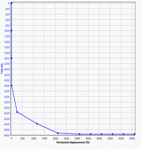
Figure 2 displays a true Vertical Depth (TVD) and Horizontal Displacement graph showing the depth of the well being drilled. TVD refers to measuring from the surface to the bottom of the borehole (or anywhere along its length) in a straight perpendicular line. It is important for well integrity to avoid damage and plan wells by designing well trajectories. Horizontal displacement (HD) is the distance the well was built horizontally after deviating from the vertical path. The graph shows that there is a positive correlation between TVD and HD. This means that as the HD of a wellbore increases, the TVD of the wellbore also increases. Interpreting this chart helps us determine the depth of our wellbore and plan the trajectory to achieve our desired objective.
Figure 2. True vertical depth vs. horizontal displacement
Figure 3. The perforation
Figure 3 shows the perforation drawing above shows the drawing of the bottom of the well with the perforations in red, the area damaged by the drilling fluid in orange, the undamaged area in yellow, the drilled hole in brown, the brine from the perforation gun in blue and the cement from the cementation of the ring in gray. Csg EH refers to the inside diameter of casing and tubes used in oil and gas wells. Casing and tubing are pipes installed in the wellbore to provide structural support, prevent the well from collapsing, and allow oil and gas production. The diameter of the casing and tubing is an important factor in determining the production rate of a well. Larger diameter housing and tubing will allow for greater flow of oil and gas. However, a larger diameter housing and tube will also be more expensive to install. A deeper well will require larger diameter casing and tubing to accommodate the higher pressure and temperature of the formation fluids. A well with a higher expected production rate will also require larger diameter casing and tubing to allow for a greater flow of oil and gas (Figure 4).
Figure 4. Casing and tubing
The AOF here in in2/ft is called an annular overflow filter. In drilling operations, an annular overflow filter (AOF) is a filtration device installed in the annular space between the casing and manifold of a wellbore. It is used to remove contaminants from drilling fluid and prevent them from entering the wellbore and potentially damaging the formation. AOF also helps protect the housing and tubes from corrosion.
4.2 PVT results
To analyze the thermodynamic parameters, we represented a phase diagram of our reservoir with the following lines: the dew line, the bubble line, the water line, the ice line and the hydrate line.
The dew line is the point on the graph where the first gas bubbles appear and the last drop of liquid disappears. The bubble line is the point on the graph where the first drop of liquid appears and the last bubble of gas disappears.
The water line represents the limit between the two-phase region (where the liquid and vapor phases coexist) and the single-phase vapor region. It indicates the minimum pressure required for the fluid in the tank to exist as vapor at a given temperature. The water line is important for understanding the behavior of reservoir fluids during production. If the tank pressure is lower than the water line, the fluid in the tank will condense into a liquid, which can reduce the flow of oil and gas to the well. This is called retrograde condensation.
The ice line represents the boundary between the two-phase region (where ice and liquid water coexist) and the single-phase liquid water region. It indicates the minimum temperature required for the reservoir fluid to exist as liquid water at a given pressure. Below the ice line, the reservoir fluid exists as single-phase liquid water, while above the ice line it exists as a two-phase mixture of ice and liquid water. The ice line is important for understanding the behavior of reservoir fluids during production, particularly in subsea environments where the reservoir temperature may be close to the freezing point of water. If the reservoir temperature drops below the ice line, the reservoir fluid will freeze and turn into ice, which can plug the wellbore and prevent the flow of oil and gas. This is called hydrate formation.
The hydrate line represents the boundary between the two-phase region (where the hydrate and vapor phases coexist) and the single-phase vapor region. It indicates the minimum pressure required for the fluid in the reservoir to form hydrates at a given temperature. Above the hydrate line, the reservoir fluid exists as a single-phase vapor, while below the hydrate line, it exists as a two-phase mixture of hydrate and vapor. Hydrates are a solid crystal structure that forms when water molecules combine with gas molecules, such as methane or ethane, under high pressure and low temperature. Hydrate formation can be a major problem in natural gas production because it can clog wellbore and pipelines, reducing or even stopping the flow of gas.
The critical point phase diagram is a graphical representation of the thermodynamic relationship between temperature, pressure, and volume of a substance. It is used to understand the behavior of a substance as it transitions between different phases, for example from a liquid to a gas or from a gas to a solid. The critical point is the point in the phase diagram where the liquid and gas phases are no longer distinguishable. At the critical point, the substance exists as a single phase called a supercritical fluid. Supercritical fluids possess properties of both liquids and gases, such as the ability to dissolve solids like gases and the ability to flow like liquids.
Figure 5. Phase diagram
In the context of a phase diagram for a reservoir fluid, the flash point is generally not represented as a specific line or curve. Rather, the flash point is a temperature at which the vapor pressure of the reservoir fluid is sufficient to form an flammable mixture with air in the presence of an ignition source. This means that the liquid in the tank is more likely to ignite and burn at temperatures above its flash point. Flash point is an important safety factor for handling and storing reservoir fluids, especially those with lower flash points. It is also important to understand the behavior of reservoir fluids during production, as flashes can occur when reservoir fluid pressure is reduced, potentially leading to the formation of flammable vapors. The figure below represents all of the different lines.
Figure 5 shows the representation of the different lines leads us to the thermodynamic parameters below.
a) Temperature profile
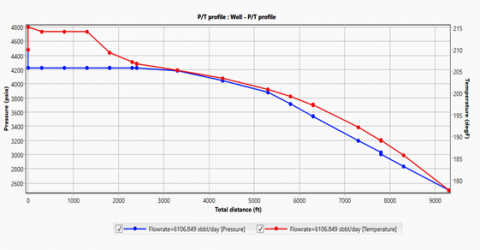
Figure 6 describes the evolution of the temperature as a function of the measured depth. The relationship between temperature and measured depth (MD) in an oil well is usually represented by a temperature gradient curve. This curve shows how temperature changes with depth. The temperature gradient curve is generally based on the geothermal gradient, which is the average rate at which temperature increases with depth in a given region. The difference between the temperature and the output of the ambient temperature segment is that the latter represents the formation temperature and the other the production temperature. Production temperature increases with depth, but based on the profile, the optimal production temperature will be around 180 degF at a depth of 7,500 feet.
Figure 7 presents the pressure profile shows that as the depth increases, the pressure does not decrease inside the well.
Figure 6. Well-P/T profile
b) Pressure profile
Figure 7. Well-P/T profile (pressure)
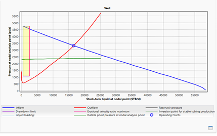
Figure 8 is a well performance graph showing two curves: the VLP curve in red and the IPR curve in blue. They are used to determine the operating point during production. Our well has an operating point of (16568.15; 3321.165).
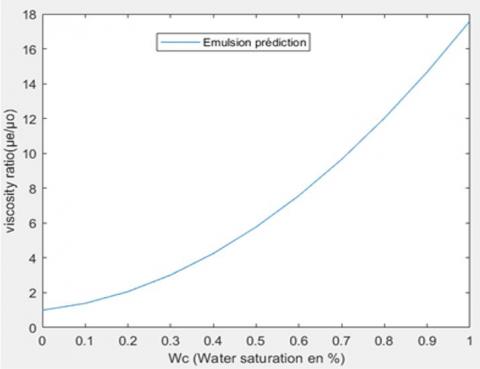
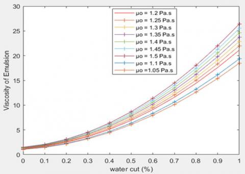
The viscosity ratio has a linear relationship with the water cut. As the viscosity ratio increases the water cut increases. This is because in this case the higher the viscosity of the fluid the higher the amount the water produced. Figures 9 to 12 shows the viscosity at different pressures and the water content of the fluid.
Figure 8. VLP vs. IPR
Figure 9. Viscosity vs. Water saturation
Figure 10. Viscosity vs. Water cut
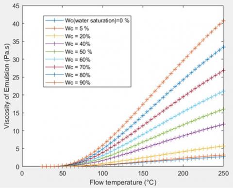
Figure 11. Viscosity vs. Flow temperature
Figure 12. Heat transfer coefficient vs. Inside radius
The viscosity of emulsion represents the amount of oil containing droplets of waters. Here we have the viscosity of oil in Pa.s and the percentage of water present at various stages.
The higher the viscosity of emulsion the higher its water cut. Hence from theses graphs we can see various the linear variations with the amount water produced.
The Higher the flow temperature the higher the viscosity of emulsion. These graph enables us to make a choice on the parameters at which we should producing to avoid paraffins accumulation. From these graphs, we can choose a flowing temperature for our producing fluid and hence the viscosity of emulsion of our producing fluid. These will enable us to choose the amount of water we are ready to produce.
These parameters are better established by the production engineer base on equipment’s on the surface.
This graph helps to determine the type of flow: laminar or turbulent. For laminar flow as the heat coefficient increases the rc and rt deceases. This influence on the heat transfer by convection. For conduction it depends on the material use for the production of the fluid. As the turbulent flow, it depends on other complex parameters.
This paper presents the results of an attempt to classify and provide calibrated correlations for crude oils in offshore horizontal wells in the RIO DEL REY region of Cameroon. The analysis is based on field data from well EKM-032. This study first gives a brief introduction to the main crude oil properties shown by the reservoir. Then, different criteria are applied to classify the PVT samples showing the impact of the data on production as well as the influence of cementing. The results show a global understanding of the PVT behaviour of crude oil in offshore horizontal wells and the development of a predictive model that can be used to optimise crude oil production. They allow a better optimisation of oil exploitation in different sites. n integration of the different modes of heat transfer could improve the results.
I would like to acknowledge the wonderful time spent at P2ST (Petroleum Services and Software Trainning ) with all the facility who permit me to finalize this work. I would also like to thank Prof B.R. Nana Nbendjo for their contributions.
|
T |
Temperture, °K |
|
|
V |
Volume, m3 |
|
|
P |
Pressure, Pa |
|
|
K |
Thermal conductivity, W.m-1. K-1 |
|
|
Greek symbols |
||
|
$\rho_0$ |
Oil density, kg. m-3 |
|
|
$\beta$ |
Thermal expansion coefficient, K-1 |
|
|
$\phi$ |
Solid volume fraction |
|
|
$\Theta$ |
Dimensionless temperature |
|
|
$\mu_{\mathrm{e}}$ |
Emulsion |
|
|
Subscripts |
||
|
$h_c$ |
Heat transfer |
|
|
F |
Fluid (pure water) |
|
|
nf |
Nanofluid |
|
[1] Babusiaux, D. (2000). Eléments pour l'analyse des évolutions des prix du brut. Cahiers de l’Economie, Série Analyses et synthèses, n° 42. 2000. hal-02460816
[2] Ayala H,L.F., Dong, T. (2015). Thermodynamic analysis of thermal responses in horizontal wellbores. Journal of Energy Resources Technology, 137(3): 032903. https://doi.org/10.1115/1.4028697
[3] Byregowda, G., Govindaswamy, R., Shivashankaran, V. (2023). Influence of open area ratio in distributor on wall to bed heat transfer coefficient from a single horizontal tube to fluidized bed of large particles. International Journal of Heat & Technology, 41(6): 1427-1432. https://doi.org/10.18280/ijht.410604
[4] Cheng, Q., Cao, G., Bai, Y., Liu, Y. (2024). The effect of crude oil stripped by surfactant action and fluid free motion characteristics in Porous Medium. Molecules, 29(2): 288. https://doi.org/10.3390/molecules29020288
[5] Li, B., Guo, Z., Du, M., Han, D., Han, J., Zheng, L., Yang, C. (2024). Research status and outlook of mechanism, characterization, performance evaluation, and type of pour point depressants in waxy crude oil: A review. Energy & Fuels, 38(9): 7480-7509. https://doi.org/10.1021/acs.energyfuels.3c04555
[6] Zhang, T., Li, Y., Li, C., Sun, S. (2020). Effect of salinity on oil production: Review on low salinity waterflooding mechanisms and exploratory study on pipeline scaling. Oil & Gas Science and Technology-Revue d’IFP Energies Nouvelles, 75: 50. https://doi.org/10.2516/ogst/2020045
[7] Ramey Jr, H.J. (1962). Wellbore heat transmission. Journal of Petroleum Technology, 14(04): 427-435. https://doi.org/10.2118/96-PA
[8] Li, G., Yang, M., Meng, Y., Wen, Z., Wang, Y., Yuan, Z. (2016). Transient heat transfer models of wellbore and formation systems during the drilling process under well kick conditions in the bottom-hole. Applied Thermal Engineering, 93: 339-347. https://doi.org/10.1016/j.applthermaleng.2015.09.110
[9] Zhang, M. (2023). Enhanced estimation of thermodynamic parameters: A hybrid approach integrating rough set theory and deep learning. International Journal of Heat & Technology, 41(6): 1587-1595. https://doi.org/10.18280/ijht.410621
[10] Cao, Z., Li, P., Li, Q., Lu, D. (2020). Integrated workflow of temperature transient analysis and pressure transient analysis for multistage fractured horizontal wells in tight oil reservoirs. International Journal of Heat and Mass Transfer, 158: 119695. https://doi.org/10.1016/j.ijheatmasstransfer.2020.119695
[11] Yoshioka, K., Zhu, D., Hill, A.D., Dawkrajai, P., Lake, L.W. (2007). Prediction of temperature changes caused by water or gas entry into a horizontal well. SPE Production & Operations, 22(04): 425-433. https://doi.org/10.2118/100209-PA
[12] Li, Z., Zhu, D. (2010). Predicting flow profile of horizontal well by downhole pressure and distributed-temperature data for waterdrive reservoir. SPE Production & Operations, 25(03): 296-304. https://doi.org/10.2118/124873-PA
[13] Alves, I.N., Alhanati, F.J.S., Shoham, O. (1992). A unified model for predicting flowing temperature distribution in wellbores and pipelines. SPE production Engineering, 7(04): 363-367. https://doi.org/10.2118/20632-PA
Arnold, F.C. (1990). Temperature variation in a circulating wellbore fluid. Journal of Energy Resources Technology, 112(2): 79-83. https://doi.org/10.1115/1.2905726
[14] Sharafutdinov, R.F., Kanafin, I.V., Khabirov, T.R. (2019). Numerical investigation of the temperature field in a multiple-zone well during gas-cut oil motion. Journal of Applied Mechanics and Technical Physics, 60(5): 889-898. https://doi.org/10.1134/S0021894419050122
[15] Yang, M., Tang, D., Chen, Y., Li, G., Zhang, X., Meng, Y. (2019). Determining initial formation temperature considering radial temperature gradient and axial thermal conduction of the wellbore fluid. Applied Thermal Engineering, 147: 876-885. https://doi.org/10.1016/j.applthermaleng.2018.11.006
[16] Zhang, R., Li, J., Liu, G., Yang, H., Jiang, H. (2019). Analysis of coupled wellbore temperature and pressure calculation model and influence factors under multi-pressure system in deep-water drilling. Energies, 12(18): 3533. https://doi.org/10.3390/en12183533
[17] Ugueto C.G.A., Huckabee, P.T., Molenaar, M.M., Wyker, B., Somanchi, K. (2016). Perforation cluster efficiency of cemented plug and perf limited entry completions; Insights from fiber optics diagnostics. In SPE Hydraulic Fracturing Technology Conference and Exhibition (p. D021S006R002). SPE. The Woodlands, Texas, USA, 9-11. https://doi.org/10.2118/179124-MS
[18] Fadairo, A.A. (2018). Modelling scale saturation around the wellbore for non-Darcy radial flow system. Egyptian Journal of Petroleum, 27(4): 583-587. https://doi.org/10.1016/j.ejpe.2017.08.009
[19] Hajirezaie, S., Wu, X., Peters, C.A. (2017). Scale formation in porous media and its impact on reservoir performance during water flooding. Journal of Natural Gas Science and Engineering, 39: 188-202. https://doi.org/10.1016/j.jngse.2017.01.019
[20] Droste, D., Lindner, F., Mundt, C., Pfitzner, M. (2013). Numerical computation of two-phase flow in porous media. In Proceedings of the 2013 COMSOL Conference in Rotterdam, Stockholm, pp. 52-57.