Yayun Fan*![]() | Weifeng Wu
| Weifeng Wu![]()
© 2024 The authors. This article is published by IIETA and is licensed under the CC BY 4.0 license (http://creativecommons.org/licenses/by/4.0/).
OPEN ACCESS
With the widespread application of composite materials in various industrial fields, accurate prediction of their thermal conductivity has become crucial. Traditional models, based mainly on equilibrium thermodynamics, fail to adequately describe the thermal behavior of composite materials under non-equilibrium conditions. This paper introduces a novel thermal conductivity prediction model based on non-equilibrium thermodynamics, focusing on entropy production adjustments and thermal conductivity prediction considering entropy production. By thoroughly analyzing the microstructure and interface characteristics of composite materials, this study aims to enhance the accuracy of thermal conductivity predictions and provide theoretical support for efficient thermal management of composite materials. The results indicate that this model effectively predicts the thermal conductivity of composite materials under non-equilibrium conditions, offering high practical value.
composite materials, non-equilibrium thermodynamics, thermal conductivity prediction, entropy production adjustment, microstructure analysis
In modern engineering and technology fields, composite materials are widely used in aerospace, automotive manufacturing, and electronic devices due to their superior mechanical properties and optimized thermal performance [1-4]. The thermal conductivity of composite materials not only affects the performance of the materials themselves but also directly relates to the thermal stability and energy efficiency of the entire system [5, 6]. Traditional methods of predicting thermal conductivity are often based on the principles of equilibrium thermodynamics. However, in practical applications, composite materials are often in a non-equilibrium state, which requires a more accurate theoretical foundation for the study of their thermal behavior.
As technology advances and material science deepens, non-equilibrium thermodynamics provides a new perspective for analyzing and predicting the thermal behavior of materials under non-equilibrium conditions [7-10]. By considering the impact of entropy production, it is possible to describe and predict changes in the thermal conductivity of composite materials in actual use environments, thereby guiding more efficient material design and application more accurately [11, 12]. Furthermore, non-equilibrium thermodynamics has potential research significance and practical value in improving the efficiency and reliability of thermal management systems.
However, although non-equilibrium thermodynamics provides a theoretical basis for understanding and predicting material thermal behavior, existing research methods still have some limitations when applied to composite materials [13-15]. Especially in terms of entropy production adjustment, traditional models often ignore or simplify the impact of the microstructure and interface effects inside composite materials on thermal conduction, resulting in predictions that significantly deviate from real application scenarios. These shortcomings limit the wide application and promotion of the model in industrial applications [16-21].
This paper aims to propose a new thermal conductivity prediction model for composite materials based on non-equilibrium thermodynamics, focusing on the entropy production adjustment and thermal conductivity prediction considering entropy production. By introducing a more detailed analysis of microstructures and interface characteristics, this study not only enhances the accuracy of the model's predictions but also provides theoretical support and methodological guidance for thermal management and application optimization of composite materials. The research outcomes will contribute to further development of composite material technology in high-demand industrial applications.
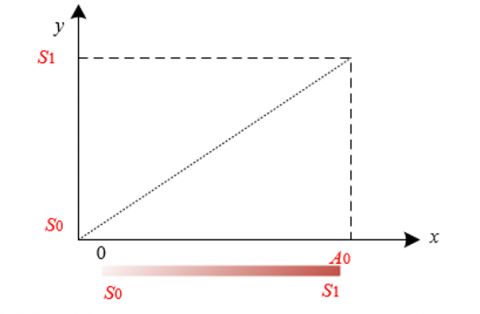
Non-equilibrium thermodynamics, particularly Onsager's reciprocal relations and their subsequent developments, provide a crucial theoretical foundation for understanding and describing irreversible processes. This theory has been proven extremely valuable in dealing with the thermal behavior of classical systems. However, for special systems such as composite materials, due to the complexity of their internal structures and the specificity of different material interfaces, standard expressions of entropy production often fail to accurately capture the generation and evolution of entropy during heat transfer processes. In the contemporary field of material science, especially in the thermal management and high-efficiency applications of composite materials, the traditional Fourier law of heat conduction has shown limitations. This is mainly because it assumes that the propagation speed of thermal disturbances is infinitely large, leading to inaccurate predictions of thermal behavior under modern technological scenarios such as high-power or ultra-short time laser heating. Additionally, the possibility of negative entropy production values in standard entropy expressions, considering time derivative correction items as seen in the C-V model and DPL model, also exposes areas needing further correction and refinement. Figure 1 shows an example of a non-equilibrium state in non-equilibrium thermodynamics.
Figure 1. Example of a non-equilibrium state in non-equilibrium thermodynamics
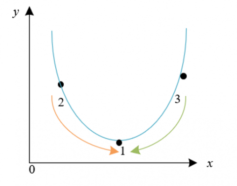
Figure 2. Schematic of the principle of minimum entropy production in the heat transfer process of composite materials
Addressing these issues, this paper focuses on entropy production corrections during the heat transfer process of composite materials based on non-equilibrium thermodynamics. This correction considers the unique internal structure and complex interactions at the multiphase interfaces of composite materials, introducing new theories from extended irreversible thermodynamics based on the principle of minimum entropy production, such as the second-order correction of heat flow, to ensure that entropy production is always positive, and it more accurately describes and predicts the thermal behavior of composite materials under extreme conditions. This specific modification of the entropy production expression reflects the fundamental differences in thermal conduction behavior between composite material systems and other material systems, not only providing theoretical innovation but also significantly enhancing the accuracy and reliability of the model in practical applications. Figure 2 provides a schematic of the principle of minimum entropy production in the heat transfer process of composite materials.
Thermal mass theory provides a revolutionary perspective for understanding and describing heat conduction in composite materials, treating heat as a "thermal mass" with a certain mass, whose movement can be simulated using the principles of fluid dynamics. This concept is particularly suitable for composite material systems, as their porous and multiphase structures make the behavior of heat transfer similar to the flow of thermal mass fluids in porous media. Within the framework of non-equilibrium thermodynamics research, by introducing heat conservation and momentum conservation equations and adjusting the entropy production expression to include the flow characteristics of thermal mass, the constructed model can more accurately predict and describe the heat conduction phenomena of composite materials under non-equilibrium thermodynamics conditions. Let ∇ be the gradient operator, s be time, S be temperature, ϑ represent density, and specific heat capacity be denoted by Z, with the specific formulas as follows:
$\frac{\partial \vartheta_g}{\partial s}+\nabla \cdot\left(\vartheta_g i_g\right)=0$ (1)
$\frac{\partial\left(\vartheta_g i_g\right)}{\partial s}+\vartheta_g\left(i_g \nabla\right) \cdot i_g+\nabla o_g+d_g=0$ (2)
Within this theoretical framework, it is possible to redefine four core concepts: thermal mass density, thermal mass pressure, mass flow rate of thermal mass, and the migration speed of heat or thermal mass, to better adapt to the unique properties and needs of composite materials.
In the thermal mass theory of composite materials, thermal mass density is defined as the equivalent mass corresponding to the amount of heat per unit volume. This includes not only the traditional concept of thermal energy density but also considers the influence of the internal structure of the material on the storage and transfer capacity of thermal energy. The heterogeneity of composite materials means that thermal mass density can vary significantly across different areas, which is crucial for predicting thermal behavior. The expression is:
$\vartheta_g=\frac{\vartheta Z S}{z^2}$ (3)
Thermal mass pressure describes the internal pressure generated during the migration of heat within a thermal mass fluid. In composite materials, due to different components' thermal responses, thermal mass pressure is influenced not only by temperature gradients but also by material interfaces and microstructural effects. This pressure helps describe the non-uniform transfer of heat in complex structures. The expression is:
$o_g=\varepsilon \vartheta_g Z S=\frac{\varepsilon \vartheta(Z S)^2}{z^2}$ (4)
In composite materials, the mass flow rate of thermal mass is defined as the amount of thermal mass passing through a specific cross-section per unit of time. It reflects not only the speed of heat transfer but also considers how the microstructural features and interface effects of the material affect the dynamic transfer of heat. This is particularly important for analyzing and designing thermal management systems for composite materials. The expression is:
$\vartheta_g i_g=\dot{l}_g=w$ (5)
The migration speed of heat or thermal mass in composite materials refers to the rate at which thermal mass propagates through the material. This definition goes beyond the traditional heat diffusion speed to include non-uniform and nonlinear effects caused by the internal structure and phase interfaces of the material. Correctly assessing this speed is crucial for predicting and controlling the thermal behavior of composite materials under high power or extreme temperature conditions. The expression is:
$i_g=\frac{w}{\vartheta Z S}$ (6)
Considering the porosity and phase interface characteristics of composite materials, it is necessary to define the motion parameters of the thermal mass fluid, including thermal mass density, thermal mass pressure, and thermal mass flow rate. At this stage, a model for calculating thermal mass resistance will also be established, where the magnitude of the resistance is proportional to the flow rate of the thermal mass. This is determined through comparison of experimental data and theoretical analysis. This resistance model needs to reflect the hindering effects of thermal mass within composite materials and consider the impact of temperature gradients and internal structural heterogeneity on heat conduction. The expression is:
$d_g=\alpha i_g$ (7)
Next, by neglecting the spatial inertial forces in the momentum equation, the universal heat conduction law is reduced to Fourier's law, which is more suitable for conditions of low-speed thermal mass flow. This step is critical as it allows the widely accepted and implemented Fourier heat conduction model to be used to approximate the heat conduction behavior in composite materials. Additionally, this simplified model can also use the heat conduction equation to obtain the resistance coefficient under small velocity conditions, which is crucial for ensuring the practicality and accuracy of the thermal mass theory in composite materials. Assuming the resistance coefficient obtained under small velocity conditions is α=2εZ(ϑZS)2/(jz2), the thermal mass resistance is represented by dg=2εϑZ2Sw/(jz2), the characteristic time by πSL=j/2εoMZ2, and the thermal wave speed by (x/πSL)1/2. Ignoring only the spatial inertial forces in the momentum equation yields the following thermal wave equation:
$\pi_{S L} \frac{\partial^2 S}{\partial s^2}-x \frac{\partial^2 S}{\partial a^2}+\frac{\partial S}{\partial s}=0$ (8)
Finally, the calculation of the entropy production rate is accomplished by dividing the rate of thermal mass energy dissipation by temperature. In composite materials, the rate of thermal mass energy dissipation is the product of resistance and the flow rate of thermal mass. Due to the complexity of the internal structure and the presence of multiphase interfaces in composite materials, this step particularly focuses on how to adjust the entropy production expression to adapt to the heat wave transmission phenomenon in complex media. This adjustment ensures that entropy production always remains positive, while also reflecting the unique heat conduction characteristics of composite materials, providing a more precise and adaptable model compared to traditional methods in other material systems. The formula for calculating the rate of thermal mass energy dissipation is:
$\begin{aligned} & \dot{q}=d_g i_g=\alpha i_g^2=\frac{2 \varepsilon(\vartheta Z S)^2}{j z^2} i_g^2 =\frac{2 \varepsilon Z S^2}{z^2} \frac{w^2}{j S^2}\end{aligned}$ (9)
Thus, the revised formula for calculating the entropy production rate is:
$\delta^s=\frac{\dot{q}}{S} \frac{z^2}{2 \varepsilon Z S}=\frac{w^2}{j S^2}$ (10)
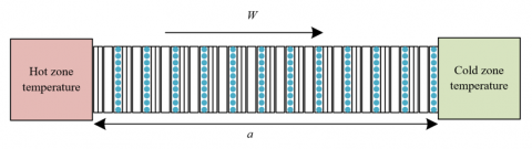
With the increasing application of composite materials in fields such as aerospace, the accurate prediction of their thermal performance has become particularly important. Conventional methods for predicting the thermal conductivity of laminated plates rely on extensive empirical data and sample testing, which are inefficient in the rapid iteration and optimization design processes. Moreover, the high anisotropy and designability of composite materials make it difficult to accurately predict their thermal conductivity under different conditions based solely on empirical data. Therefore, it is necessary to study a method for predicting the thermal conductivity of composite materials that considers entropy production during the heat transfer process, aiming to provide a more scientific and technologically advanced solution to support rapid iteration of structural design and comprehensive assessment of composite material performance. Figure 3 shows the model of heat transfer in a single direction for composite materials.
Figure 3. Model of heat transfer in a single direction for composite materials
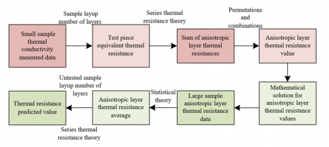
This paper proposes a method for predicting the thermal conductivity of composite materials considering entropy production during the heat transfer process. Fundamentally, this new method integrates non-equilibrium thermodynamics theory into the thermal transfer analysis of composite materials, particularly by modifying and considering the entropy production during the heat transfer process to improve prediction accuracy. Traditional models often overlook the non-equilibrium effects in complex heat transfer processes, such as thermal wave phenomena and the nonlinear distribution of heat, which are particularly important in composite materials. By introducing entropy production correction, this method can more accurately simulate the transfer of heat across different levels and directions of the material, and reflect the changes in thermal behavior caused by complex microstructures and differences in layup order. This approach relies on less experimental data, predicting thermal conductivity through theoretical analysis and mathematical modeling, greatly enhancing the flexibility and efficiency of the design. Figure 4 provides the process flow for the prediction method of single-direction thermal conductivity for composite materials.
Figure 4. Process flow for the prediction method of single-direction thermal conductivity for composite materials
3.1 Prediction method for Z-direction thermal conductivity
In the prediction of thermal conductivity of composite materials considering entropy production, it is first necessary to precisely measure the equivalent thermal resistance of each sample. Since the temperature rise in the Laser Flash Analysis (LFA) test is very small, it is assumed that the temperature of each layer remains the same during the instantaneous heating process, and thus layers at the same angle have the same thermal conductivity and thermal resistance. At this point, the thermal resistance of layers at different angles can be added according to the series thermal resistance theory to obtain the total equivalent thermal resistance of the sample. Assuming the thickness of the composite sample is represented by f, the following formula provides the calculation of equivalent thermal resistance for each measured thermal conductivity data Jz:
$E_s=f / J_r$ (11)
Assuming the equivalent thermal resistance of the composite sample is represented by Es, the total number of layers of the current angle layup in the sample is represented by V, and the thermal resistance of the corresponding angle layer is represented by E, eliminating single-layer thickness it is considered that E=J-1, the thermal conductivity of that angle layer is represented by J, at this time Es=Vs/Jr, where the sample layup number of layers is represented by Vs. The total equivalent thermal resistance can be calculated using the following formula:
$E_s=V_0 E_0+V_{45} E_{45}+V_{-45} E_{-45}+V_{90} E_{90}$ (12)
Based on the obtained data for anisotropic layer thermal resistance, a set of quartic equations can be established, where the unknowns are the thermal resistances E0, E45, E-45, E90 of different angle layers. These equations are derived from empirical data at the same temperature of different samples, and at least four sets of data are required to solve for the four unknowns. Assuming the number of empirical data sets at the current temperature is represented by v, combining these equations can form Z4v possible sets of equations, each first set of equations being of the form shown below:
$\left\{\begin{array}{l}V_0^1 E_0+V_{45}^1 E_{45}+V_{-45}^1 E_{-45}+V_{90}^1 E_{90}=E_s^1 \\ V_0^2 E_0+V_{45}^2 E_{45}+V_{-45}^2 E_{-45}+V_{90}^2 E_{90}=E_s^2 \\ V_0^3 E_0+V_{45}^3 E_{45}+V_{-45}^3 E_{-45}+V_{90}^3 E_{90}=E_s^3 \\ V_0^4 E_0+V_{45}^4 E_{45}+V_{-45}^4 E_{-45}+V_{90}^4 E_{90}=E_s^4\end{array}\right.$ (13)
According to the principles of linear algebra, the values of E0, E45, E-45, E90 can be determined by solving a system of linear equations in the form of XA=Y. A prerequisite for this step is that the coefficient matrix X must be full rank. Solving each set of equations yields a set of thermal resistances. During the solution process, it is necessary to consider the physical meaning of thermal resistance, ensuring that all solutions are greater than zero to reflect the actual physical processes. After determining all mathematically valid combinations of thermal resistance, further filter out those that make physical sense and calculate the average values of the anisotropic layer thermal resistances to obtain E0, E45, E-45, and E90. These averages are based on empirical data and consider the effects of entropy production under non-equilibrium conditions, thus providing a more reliable basis for prediction. The formula for predicting thermal resistance is:
$E_o=V_0 \bar{E}_0+V_{45} \bar{E}_{45}+V_{-45} \bar{E}_{-45}+V_{90} \bar{E}_{90}$ (14)
Finally, based on the layup order and the number of layers V of the sample to be tested, the equivalent thermal resistance of the layered composite material is calculated again using the series thermal resistance theory, combined with the number of layers V of the sample, to predict the Z-direction thermal conductivity. This step not only relies on the classic series thermal resistance model but also incorporates considerations of entropy production, making the prediction more consistent with the actual thermal conduction characteristics of composite materials under working conditions. The calculation formula is:
$J_{r d}=V / E_o$ (15)
3.2 Prediction method for X/Y direction thermal conductivity
For predicting the thermal conductivity in the X/Y directions, the thermal conductivity of composite laminated plates at different angles of layers (-45°, 45°, 0°, and 90°) is first measured. Due to the limitations of the LFA test, the measured thermal conductivity data only represent the thermal behavior of some layers within the detection area, rather than the overall equivalent thermal conductivity along the X or Y directions. This requires a detailed analysis of the empirical data to ensure their correct use in the mathematical model. Assuming the number of layers at a given angle is represented by V, the cross-sectional area of the corresponding angle layer is represented by X, the thickness of the sample by a, and the total cross-sectional area of the sample by XTO, the equivalent thermal conductivity of the composite sample is represented by Jr, and the temperature difference between the hot and cold ends by ΔS. Based on the consistency of the total heat transferred, the following equation can be established:
$\begin{aligned} & V_0 X_0 J_0\left(\frac{\Delta S}{a}\right)+V_{45} X_{45} J_{45}\left(\frac{\Delta S}{a}\right)+V_{-45} X_{-45} J_{-45}\left(\frac{\Delta S}{a}\right)+ V_{90} X_{90} J_{90}\left(\frac{\Delta S}{a}\right)=X_{T O} J_e\left(\frac{\Delta S}{a}\right)\end{aligned}$ (16)
Assuming the proportion of each angle layer in the total number of layers is represented by e, the equation can be simplified as follows:
$J_e=e_0 J_0+e_{45} J_{45}+e_{-45} J_{-45}+e_{90} J_{90}$ (17)
Using the measured thermal conductivity data, construct a parallel heat transfer model for the X/Y directions. This model needs to consider the specific configuration of the composite material layers, as the proportion of different angle layers directly affects the thermal conductivity in the X or Y directions. At this time, it is necessary to consider the relative position and proportion of each layer within the detection area to accurately calculate the equivalent X/Y directional thermal conductivity.
For pure single-angle laminates (such as pure 0° or pure 45° layers), since the total area of the sample equals the total area of that angle layer, the calculation process for thermal conductivity can be simplified. Here, the thermal conductivity calculation can directly apply the established parallel heat transfer model, deriving the thermal conductivity of a single-angle layer from empirical data. Assuming the thermal conductivity of the ϕ angle layer is represented by Jϕ, the simplified formula for predicting the thermal conductivity of a single-angle ϕ layer sample is given by:
$J_r=J_{\varphi}$ (18)
Finally, using data obtained from single-angle layers, predict the X/Y directional thermal conductivity of conventional layering method samples. In composite materials, the X and Y directional thermal conductivity of a specific angle layer might be the same as that of another angle's layer. For example, the X-direction thermal conductivity of a 0° layer and the Y-direction thermal conductivity of a 90° layer are the same. This symmetry makes the actual testing and prediction more convenient and accurate. This step particularly considers the entropy production in non-equilibrium thermodynamics, ensuring that the prediction of thermal conductivity is not only based on empirical data but also reflects the dynamic thermal behavior of composite materials under non-equilibrium conditions.
Analysis of the data from Table 1 shows the thermal behavior characteristics of composite materials within different temperature ranges, in terms of thermal mass density, thermal mass pressure, thermal mass resistance, and their uncertainties. For example, Sample Number 1 has a thermal mass density of 3.2514 kg/m³ with a relatively low uncertainty of 0.2784%, demonstrating stable thermal mass properties within the temperature range of 262-312 K. The uncertainties of thermal mass pressure and thermal mass resistance are generally higher, such as the thermal mass pressure uncertainty of Sample 5, reaching 0.4678%, reflecting greater variability in the internal thermal stresses and resistances of composite materials under complex temperature conditions. These data support the necessity of precise measurement of thermal mass theoretical parameters in composite materials, as well as the importance of entropy production correction within the framework of non-equilibrium thermodynamics. The data in the table reflects the performance of different samples under a wide range of temperature conditions and heat migration speeds, showing significant differences in heat transfer characteristics and emphasizing the impact of considering changes in the internal microstructure of composite materials on predicting thermal conductivity.
Table 1. Comparison of entropy production correction results in the heat transfer process of composite materials
|
Sample Number |
Thermal Mass Density |
Uncertainty % |
Thermal Mass Pressure |
Uncertainty % |
Thermal Mass Resistance |
Uncertainty % |
Temperature Range /K |
|
|
Mass Flow Rate of Thermal Mass |
Migration Speed of Heat or Thermal Mass |
|||||||
|
1 |
3.2514 |
0.2784 |
3.1205 |
0.0714 |
4.742 |
0.1785 |
262-312 |
189-356 |
|
2 |
2.9852 |
0.6754 |
3.3215 |
0.1895 |
4.722 |
0.4215 |
265-300 |
321-357 |
|
3 |
2.6254 |
0.7452 |
3.1245 |
0.1523 |
4.913 |
0.4895 |
242-315 |
158-314 |
|
4 |
3.5624 |
0.3785 |
3.2652 |
0.1214 |
4.612 |
0.2236 |
256-314 |
265-389 |
|
5 |
3.3241 |
1.1245 |
3.1245 |
0.4678 |
4.715 |
0.6214 |
224-265 |
387-374 |
|
6 |
2.5625 |
0.7895 |
2.8795 |
0.2132 |
4.786 |
0.4895 |
256-314 |
245-321 |
|
7 |
2.2369 |
0.2325 |
3.6521 |
0.0452 |
4.142 |
0.1562 |
245-326 |
121-231 |
|
8 |
2.1421 |
1.1245 |
3.5698 |
0.1236 |
4.015 |
0.7256 |
254-356 |
201-289 |
|
9 |
2.4587 |
0.5784 |
2.4512 |
0.1785 |
4.526 |
0.3692 |
234-278 |
245-312 |
|
10 |
3.1256 |
0.3215 |
3.1245 |
0.0985 |
4.548 |
0.1895 |
178-789 |
268-331 |
|
11 |
2.6235 |
0.3269 |
3.2366 |
0.1142 |
4.736 |
0.1862 |
224-256 |
237-269 |
1) Z direction
2) X direction
3) Y direction
Figure 5. Distribution of relative errors between predicted and tested thermal conductivities in different directions of composite materials
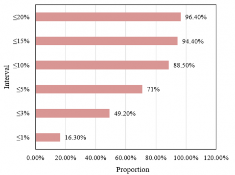
Figure 5-1 displays the distribution of relative errors between the predicted and experimental values of the thermal conductivity in the Z-direction of composite materials, where different error intervals correspond to different proportions of samples. Specifically, 16.30% of the samples have a relative error of less than or equal to 1%, meaning that over one-sixth of all test samples achieved very high prediction accuracy. As the permissible error interval increases, the proportion of samples significantly increases; for example, when the error tolerance is raised to 3%, nearly half of the samples (49.20%) have predictions very close to the actual measurements. Further expanding to within a 5% error range, over seventy percent (71%) of the samples are accurately predicted, and when the error range is increased to 20%, almost all samples (96.40%) align well with the experimental values.
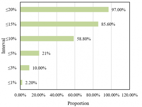
Figure 5-2 shows the distribution of relative errors between the predicted and actual values of the thermal conductivity in the X-direction of composite materials. The data shows that within a very strict error range (≤1%), only 2.20% of the samples achieved this accuracy, demonstrating the challenges of prediction within very low error intervals. When the error limit is expanded to 3%, the proportion of samples increases to 10.00%, and as the error tolerance further increases to 5%, 21% of the samples meet the prediction accuracy requirements. Within broader error intervals (≤10% and ≤15%), the pass rates of the samples significantly increase to 58.80% and 85.60%, respectively. Finally, when the permissible error reaches or is less than 20%, 97.00% of the samples meet or exceed the prediction accuracy requirements, indicating that the vast majority of samples have predictions that are consistent with experimental values.
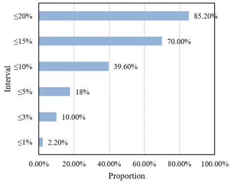
Figure 5-3 shows the data for the distribution of relative errors between predicted and actual values of the thermal conductivity in the Y-direction of composite materials. The data reveals that within a very strict error range (≤1%), the prediction accuracy is low, with only 2.20% of the samples meeting this standard. As the error limit is relaxed to 3% and 5%, the compliance rates of the samples increase to 10.00% and 18%, respectively, showing a moderate improvement in prediction accuracy. When the error range is further expanded to 10%, the compliance rate reaches 39.60%, and as the error range expands to 15% and 20%, the compliance rates significantly increase to 70.00% and 85.20%, respectively. This indicates that as the error range increases, the proportion of samples covered by the prediction model gradually increases, although the performance in lower error ranges is not particularly ideal.
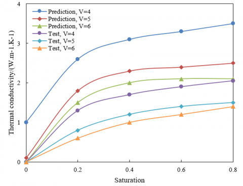
Figure 6. Thermal Conductivity of Composite Materials as a Function of Saturation
Figure 6 shows the predicted and tested values of thermal conductivity of composite materials at different corresponding layer counts (V=4, V=5, V=6) as saturation changes. From the data analysis, it can be observed that the thermal conductivity increases with saturation for both predicted and tested values. Specifically, for a layer count of V=4, the predicted thermal conductivity increases from 1 to 3.5, while the tested values rise from 0 to 2.05; for V=5, the predicted conductivity increases from 0.1 to 2.5, and the tested values from 0 to 1.5; for V=6, the predicted conductivity increases from 0 to 2.1, with tested values increasing from 0 to 1.4. This illustrates the significant impact of saturation on the thermal conductivity of composite materials and also reveals the accuracy of the prediction model in capturing the trend of conductivity changes at different layer counts.
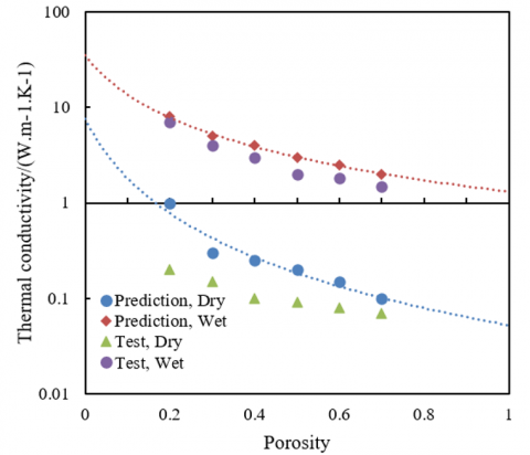
Figure 7. Changes in thermal conductivity of composite materials with porosity
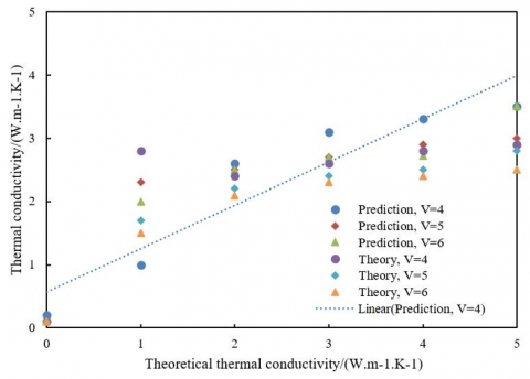
Figure 8. Comparison of theoretical and predicted thermal conductivities of composite materials
The data in Figure 7 reveals the trends in thermal conductivity of composite materials under varying porosity levels, specifically under dry and wet conditions. The data shows that thermal conductivity significantly decreases with increasing porosity under both dry and wet conditions. Under dry conditions, the predicted thermal conductivity gradually decreases from 1 to 0.1, while actual data drops from 0.2 to 0.07, showing predictions systematically higher than actual values but with a consistent trend. Under wet conditions, predicted thermal conductivity decreases from 8 to 2, and actual conductivity from 7 to 1.5, also displaying the characteristic of predictions being generally higher than actual values. Nonetheless, both effectively capture the downward trend of thermal conductivity with increasing porosity.
Figure 8 presents data comparing the predicted and theoretical thermal conductivities of composite materials across different layer counts (V=4, V=5, V=6) under multiple test thermal conductivity values. The table shows varying degrees of discrepancies between the predicted and theoretical thermal conductivities at each level. For example, at V=4, the predictions in the higher thermal conductivity range (2.6 to 3.5) are generally above the theoretical values (2.4 to 2.9). Similarly, for V=5 and V=6, the predictions also show higher values compared to theoretical values at mid to high thermal conductivities. This trend is common across all levels, indicating that the prediction model tends to overestimate at higher conductivities. Overall, the model demonstrates its effectiveness, particularly in simulating the thermal behavior at different layer counts (V values).
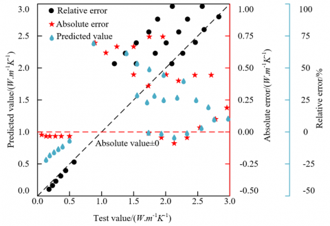
Figure 9. Comparison of predicted results and experimental test results for thermal conductivity of composite materials
Based on the data in Figure 9, the predictions of thermal conductivity of composite materials align well with experimental results in most cases, particularly when the saturation is high or low. Specifically, at low saturation levels, the absolute errors in the predicted smaller thermal conductivities are less than 0.5 W/(m-K), and at high saturation levels, where thermal conductivity is greater, the same absolute errors show relative errors between 20% and 30%. This error range is acceptable for predictions of thermal conductivity because even small absolute errors can appear relatively significant due to the inherent fluctuations in thermal conductivity of composite materials, a phenomenon commonly seen in studies of convective heat transfer coefficients.
From the analysis, it can be concluded that the prediction model based on non-equilibrium thermodynamics is practical and reliable, especially in dealing with predictions of thermal conductivity of composite materials under extreme saturation conditions. However, the model shows larger prediction errors at medium saturation levels, which may affect a comprehensive understanding and analysis of the thermal behavior of composite materials. Therefore, while the model performs stably in most situations, further improvements and refinements are needed for the prediction algorithms under medium saturation to reduce prediction errors and enhance the model's accuracy and applicability across all operating ranges. Further research and adjustment of model parameters might be crucial for optimizing prediction accuracy and expanding the model’s application scope.
This paper introduces a new prediction model for the thermal conductivity of composite materials based on non-equilibrium thermodynamics, with a focus on the impact of entropy production during the heat transfer process and explores thermal conductivity predictions considering entropy production. Through a series of experimental results, this study analyzed the effect of entropy production correction in the heat transfer process of composite materials, the distribution of relative errors between predicted and tested values of thermal conductivity in the X, Y, and Z directions, and the relationship between thermal conductivity, saturation, and porosity of composite materials. Additionally, the paper discussed in detail the comparison between theoretical and predicted values of thermal conductivity to comprehensively evaluate the effectiveness of the prediction model.
Synthesizing experimental data and analysis results, the conclusions drawn indicate that the non-equilibrium thermodynamics-based prediction model shows good reliability under conditions of low and high saturation, with absolute errors less than 0.5 W/(m-K) and relative errors between 20% to 30%. The model exhibits a stable trend in predicting thermal conductivity in the X, Y, and Z directions of composite materials, but shows larger discrepancies between predicted and experimental values at medium saturation levels and higher porosity. The research value of this paper lies in revealing the critical role of entropy production in the heat transfer of composite materials and providing a link between theory and experimental results, offering new insights into the prediction of thermal conductivity for composite materials.
However, the study still has limitations, such as significant prediction errors in the model at medium saturation levels and occasionally high predictions by the theoretical model. Additionally, due to the complexity of composite materials, the entropy production correction model may require further adjustments and optimizations. Future research directions could include improving model parameterization, further exploring the impact of entropy production under different temperatures and environmental conditions, and validating the prediction model's effectiveness in a broader range of composite material applications. Through these further studies, the accuracy and applicability of the model can be enhanced, providing more reliable guidance for engineering applications and material development.
[1] Li, Y., Lin, C., Murengami, B.G., Tang, C., Chen, X. (2023). Analyses and research on a model for effective thermal conductivity of laser-clad composite materials. Materials, 16(23): 7360. https://doi.org/10.3390/ma16237360
[2] Shen, C., Sheng, Q., Zhao, H. (2023). Predicting effective thermal conductivity of fibrous and particulate composite materials using convolutional neural network. Mechanics of Materials, 186: 104804. https://doi.org/10.1016/j.mechmat.2023.104804
[3] Ito, Y., Takanishi, K., Sakamoto, T., Fujiwara, K., Arai, H. (2023). Development of printed circuit boards with high thermal conductivity and low thermal expansion by applying cu-mo composite materials. In Advancing Microelectronics Symposium, pp. 85-89.
[4] Popov, I.A., Gortyshov, Y.F., Popov, I.A. (2023). Thermal conductivity of new carbon polymer composite materials. Russian Aeronautics, 66(3): 581-585. https://doi.org/10.3103/S1068799823030212
[5] Yu, H., Fu, J., Wu, Y., Zhang, X. (2024). Low thermal conductivity and high thermoelectric performance in Cu2Se/CuAgSe composite materials. Journal of Materials Science: Materials in Electronics, 35(6): 1-8. https://doi.org/10.1007/s10854-024-12113-6
[6] Mao, L.K., Liu, Q., Chen, H., Cheng, W. L. (2024). A novel model of the anisotropic thermal conductivity of composite phase change materials under compression. International Journal of Heat and Mass Transfer, 227: 125512. https://doi.org/10.1016/j.ijheatmasstransfer.2024.125512
[7] Yang, Y., Li, B., Che, L., Li, M., Luo, Y., Han, H. (2024). Calculation model and influence factors of thermal conductivity of composite cement-based materials for geothermal well. Geothermal Energy, 12(1): 3. https://doi.org/10.1186/s40517-024-00282-w
[8] Gay-Balmaz, F., Yoshimura, H. (2023). Systems, variational principles and interconnections in non-equilibrium thermodynamics. Philosophical Transactions of the Royal Society A, 381(2256): 20220280. https://doi.org/10.1098/rsta.2022.0280
[9] Konstantinou, P.C., Stephanou, P.S. (2023). Predicting high-density polyethylene melt rheology using a multimode tube model derived using non-equilibrium thermodynamics. Polymers, 15(15): 3322. https://doi.org/10.3390/polym15153322
[10] Pyurbeeva, E., Thomas, J.O., Mol, J.A. (2023). Non-equilibrium thermodynamics in a single-molecule quantum system. Materials for Quantum Technology, 3(2): 025003. https://doi.org/10.1088/2633-4356/accd3a
[11] Skibsted, L.H. (2024). Perspectives of non-equilibrium thermodynamics of calcium transport by caseins. European Food Research and Technology, 250(1): 15-20. https://doi.org/10.1007/s00217-023-04380-0
[12] Ruiz, M.S., Razzitte, A. (2024). Study of entropy production of magnetoelectric multiferroic materials. Journal of Electronic Materials, 53: 1600-1605. https://doi.org/10.1007/s11664-023-10876-y
[13] Chiu, C.T., Teng, Y.J., Dai, B.H., Tsao, I.Y., Lin, W.C., Wang, K.W., Hung, W.H. (2022). Novel high-entropy ceramic/carbon composite materials for the decomposition of organic pollutants. Materials Chemistry and Physics, 275: 125274. https://doi.org/10.1016/j.matchemphys.2021.125274
[14] Coşkun, A., Irmak, A.E., Altan, B., Ak, Y.S., Coşkun, A.T. (2023). Tuning the magnetic and magnetocaloric properties of a compound via mixing (1–x). La0. 67Ca0. 33MnO3+ x. La0. 67Sr0. 33MnO3 (x= 0, 0.25, 0.50, 0.75, 1): Composite materials or composite compounds? Journal of Magnetism and Magnetic Materials, 584: 171104. https://doi.org/10.1016/j.jmmm.2023.171104
[15] Al-Khazaal, A.Z. (2022). Effects of composite material fin conductivity on natural convection heat transfer and entropy generation inside 3D cavity filled with hybrid nanofluid. Journal of Thermal Analysis and Calorimetry, 147(5): 3709-3720. https://doi.org/10.1007/s10973-021-10737-y
[16] Dwivedi, S.P., Sharma, S. (2024). Synthesis of high entropy alloy AlCoCrFeNiCuSn reinforced AlSi7Mg0.3 based composite developed by solid state technique. Materials Letters, 355: 135556. https://doi.org/10.1016/j.matlet.2023.135556
[17] Xu, X., Shao, Z., Jiang, S.P. (2022). High-entropy materials for water electrolysis. Energy Technology, 10(11): 2200573. https://doi.org/10.1002/ente.202200573
[18] Chang, C.C., Brousset, T., Chueh, C.C., Bertei, A. (2021). Effective thermal conductivity of composite materials made of a randomly packed densified spherical phase. International Journal of Thermal Sciences, 170: 107123. https://doi.org/10.1016/j.ijthermalsci.2021.107123
[19] Sun, H., Shi, Y., Liu, W., Shi, W., Su, S., Xiao, Y. (2021). Theoretical prediction for effective thermal conductivity of composite materials with random structure. Acta Materiae Compositae Sinica, 38(9): 2925-2933.
[20] Li, R., Zhao, Y., Xia, B., Dong, Z., Xue, S., Huo, X., Zhang, X. (2021). Enhanced thermal conductivity of composite phase change materials based on carbon modified expanded perlite. Materials Chemistry and Physics, 261: 124226. https://doi.org/10.1016/j.matchemphys.2021.124226
[21] Li, C., Wang, M., Chen, Z., Chen, J. (2021). Enhanced thermal conductivity and photo-to-thermal performance of diatomite-based composite phase change materials for thermal energy storage. Journal of Energy Storage, 34: 102171. https://doi.org/10.1016/j.est.2020.102171