Xiaolong Cheng*![]() | Xujin Zhang | Linpeng Su
| Xujin Zhang | Linpeng Su
© 2024 The authors. This article is published by IIETA and is licensed under the CC BY 4.0 license (http://creativecommons.org/licenses/by/4.0/).
OPEN ACCESS
With the rapid development of transportation infrastructure construction, tunnels, serving as key channels through complex terrains such as mountainous regions and rivers, are confronted with numerous challenges during design and construction phases. Particularly, in tunnel projects with sharp curves, traditional design methods, lacking in-depth analysis of fluid-structure interaction (FSI) effects under navigation conditions, struggle to ensure the long-term safety and stability of tunnels. This study systematically investigates the FSI issues in sharp-curve tunnel sections under navigation conditions through numerical simulation and optimization, aiming to enhance the scientific and practical aspects of tunnel design. Initially, a numerical model suitable for the FSI analysis of sharp-curve tunnel sections was established, capable of simulating the complex interplay between fluid dynamics and tunnel structures. The forces exerted by the fluid on the tunnel structure and its dynamic response characteristics were analyzed in detail through the calculation of coupled fields of fluid dynamics and structural mechanics. Subsequently, the impact of dynamic response parameters of tunnel structures on overall performance was explored using global sensitivity analysis methods. Finally, based on multi-objective optimization theory, the design parameters of tunnel structures were optimized to achieve higher safety and economic efficiency. The methodologies and findings of this article hold significant theoretical value for the design of sharp-curve tunnel sections and provide a reliable analysis and optimization tool for similar complex engineering problems. Practical outcomes indicate that this research significantly enhances the performance of tunnel design, playing a substantial role in ensuring the safe operation of tunnel projects.
fluid-structure interaction (FSI), sharp-curve tunnels, numerical simulation, global sensitivity analysis, multi-objective optimization, tunnel design
As the modern transportation network rapidly evolves, tunnels, being integral components of transportation infrastructure, have garnered increasing attention in design and construction amidst complex geological conditions [1-3]. Particularly in sharp-curve sections such as mountainous areas and rivers, the design of tunnels not only requires ensuring structural safety and stability but also necessitates accommodating the FSI effects under navigation conditions, thereby imposing higher demands on the scientific and rational aspects of tunnel design [4, 5]. The dynamic effects of water flow and the interaction with tunnel structures in sharp-curve sections are especially complex, directly influencing the safe operation and lifespan of the tunnels [6-8]. Therefore, an in-depth analysis of the FSI phenomenon in sharp-curve tunnels under navigation conditions through numerical simulation holds significant theoretical and practical relevance for optimizing tunnel design.
Research on FSI problems has emerged as a focal point in the fields of engineering mechanics and fluid dynamics. In tunnel engineering, FSI analysis reveals the intrinsic mechanisms of interaction between water flow and tunnel structures, providing a scientific basis for the design, construction, maintenance, and safety assessment of tunnels [9]. However, due to the nonlinear nature of FSI issues in sharp-curve tunnels, along with the variability of water flow conditions and geological environments, traditional analysis methods often fall short in accuracy and reliability, failing to meet the demands for refined and personalized design [10-12].
Existing studies on FSI largely rely on simplified physical models or numerical simulations under specific boundary conditions. These methods struggle to address complex geological conditions and real-world engineering challenges [13, 14]. Particularly for sharp-curve tunnels, the transient effects of fluid, the nonlinear response of structures, and their interactions pose substantial challenges to accurate simulation [15-17]. Moreover, previous research has often overlooked global sensitivity analysis of dynamic response parameters of tunnel structures, which is crucial for the optimization of tunnel design and safety evaluation.
This study unfolds around two core sections. Firstly, advanced numerical simulation technology is utilized to delve into the FSI effects in sharp-curve tunnels under navigation conditions. By computing the coupled fields of fluid dynamics and structural mechanics, the impact of fluid on tunnel structures and their dynamic characteristics are analyzed. Secondly, through global sensitivity analysis, the extent to which dynamic response parameters of tunnel structures affect overall performance is revealed. Subsequently, based on multi-objective optimization theory, design parameters of tunnel structures are optimized to achieve higher safety and economic efficiency. The innovation of this study lies in the comprehensive application of multidisciplinary techniques, proposing a FSI analysis and optimization framework tailored for sharp-curve tunnel design. This offers solutions for similar complex engineering problems, possessing significant theoretical value and broad engineering application prospects.
To simulate the FSI phenomenon in sharp-curve tunnels under navigation conditions, high-precision finite element modeling was performed using the ANSYS Workbench platform. Initially, the Fluent module was employed to conduct a detailed calculation of the flow field within the tunnel, identifying characteristics of the sharp-curve fluid flow, including velocity distribution and pressure field. The obtained flow field pressure data, serving as load conditions, were transmitted to the Transient Structural module via a system coupling interface to solve for the tunnel structure's dynamic response under fluid dynamics effects, including deformation and stress distribution. Subsequently, the deformation of the tunnel structure was fed back into the flow field model to adjust fluid boundary conditions, ensuring accurate simulation of the tunnel structure's response on the flow field. This computational process was repeated within each time step until the flow field and structural response at the current time step converged, followed by computations for the next time step. Iterating this process allowed for the acquisition of a time-domain solution for the dynamic process of FSI in sharp-curve sections of tunnels under entire navigation conditions, thus providing more precise dynamic analysis data and optimization basis for tunnel design.
2.1 Steady-state simulation of sharp-curve tunnels
When calculating the water flow velocity in sharp-curve tunnel sections under navigation conditions, it is first necessary to collect information about the tunnel's geometric features such as length, cross-sectional shape, curve radius, etc., hydrological data such as flow rate, water level, as well as roughness information of the tunnel walls. Based on the specific conditions of the tunnel and available data, a suitable calculation method is selected. For complex situations, Computational Fluid Dynamics (CFD) simulation might be required. For simpler scenarios, formulas such as Manning or Chezy could be used. CFD, a numerical analysis tool for studying and solving fluid flow and transfer phenomena, is capable of simulating complex fluid flows, especially suited for analyzing non-uniform, unsteady flow conditions in sharp-curve tunnel sections. In CFD models, fluid flow within the tunnel is typically considered as an incompressible Newtonian fluid, described by the Navier-Stokes equations. Assuming the mass fluid density is represented by $\rho$, the change in velocity over time by $\partial V / \partial t$, the movement speed and direction of fluid by $V \nabla V$, the internal pressure gradient of the fluid by $\nabla P$, the external force acting on the fluid by $\rho g$, and the internal stress acting on the fluid by $\mu \nabla^2 V$, the following equation is obtained:
$\rho\left(\frac{\partial V}{\partial t}+V \cdot \nabla V\right)=\nabla P+\rho g+\mu \nabla^2 V$ (1)
For situations where direct CFD simulation is not feasible, physical model experiments combined with empirical formulas may be employed to estimate flow velocity, especially during the preliminary design phase. Common empirical formulas, such as the Manning formula, allow for the estimation of flow velocity based on known conditions. Assuming the average velocity of the cross-section is represented by V, the conversion coefficient by k, the Manning coefficient by n, the hydraulic radius by Rh, and the hydraulic slope by S, the following equation can be formulated:
$V=\frac{k}{n} R_h^{2 / 3} S^{1 / 2}$ (2)
In the steady-state simulation analysis of FSI in sharp-curve tunnels under navigation conditions, the pressure at the tunnel exit and the flow velocity at the entrance are initially defined. Specifically, the pressure at the tunnel exit and the flow velocity at the entrance are set. These conditions provide baseline data for comparison with subsequent fluid simulation results.
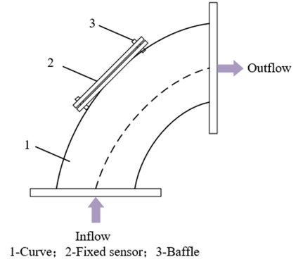
Figure 1 presents a schematic diagram of a sharp-curve tunnel under navigation conditions. Under steady-state fluid flow conditions, the pressure distribution in the straight sections of the tunnel is relatively uniform, as the fluid here is less affected by geometric structures, resulting in more stable flow and consistent pressure loss. However, as the fluid enters the sharp-curve section, the pressure field begins to change. The fluid pressure on the outer side of the curve increases, reaching a maximum value at a certain point before gradually decreasing; meanwhile, the fluid pressure on the inner side of the curve gradually decreases, reaching a minimum value before beginning to increase. This phenomenon illustrates the complexity of fluid dynamics in sharp-curve tunnel sections, particularly the secondary flows and vortices induced by the curve shape.
Figure 1. Schematic diagram of a sharp-curve tunnel under navigation conditions
From the perspective of the velocity field distribution, the flow velocity on the outer side of the tunnel's sharp curve is less than on the inner side. This is due to the guiding action of the curved wall and the result of centrifugal forces, which accelerate the fluid flow on the inner side. After the sharp-curve section, the velocity field at the exit of the curve becomes unstable due to fluid impact and disturbances, especially near the exit walls, where small-scale vortices and stagnation zones form due to the redistribution of fluid and reduction in velocity.
The FSI effects are particularly pronounced in sharp-curve tunnel sections. Due to the significant curvature changes of the tunnel's inner walls, the impact and friction of the fluid on the tunnel walls are intensified. This effect is most notable in the middle part of the sharp-curve section, resulting in the maximum deformation and stress on the tunnel walls. The greatest deformation often occurs on the outer side, where the fluid pressure is highest; while the greatest stress appears on the inner side, due to the need to resist the sharp change in the direction of fluid flow.
The response of tunnel structures under the action of fluid dynamics directly impacts the structural integrity and safety of the tunnel. In sharp-curve sections, the complexity of fluid flow exacerbates, leading to more bending and torsional deformation of the tunnel walls. To ensure the safety of the tunnel, these deformations and stress distributions must be accurately calculated, and the tunnel structure designed accordingly, to withstand these pressures without sustaining damage.
2.2 Dynamic simulation with input water hammer pressure
In the dynamic simulation analysis of FSI in sharp-curve tunnels under navigation conditions, the fluid within the tunnel can also be considered as a superposition of average pressure and water hammer pressure. Water hammer pressure arises from sudden changes in flow conditions, such as the passage of ships, rapid closing or opening of valves, generating pressure fluctuations within the fluid. These fluctuations can significantly increase local pressure in a short time. When setting the exit boundary conditions of the tunnel, the dynamic characteristics of the fluid must be considered to ensure the exit boundary conditions can reflect the characteristics of actual water hammer pressure fluctuations accurately.
Initially, the pressure fluctuations at the tunnel exit are defined. If the frequency and amplitude of water hammer pressure fluctuations at the exit are known, these data can be used to set the pressure fluctuation conditions at the tunnel exit. Given the frequency of water hammer pressure fluctuations and the rate of change, the tunnel exit pressure needs to be set to fluctuate by ±5% of the average pressure due to water hammer. This means that if the average pressure is 1000MPa, the water hammer pressure will vary between 950MPa and 1050MPa. Based on the aforementioned conditions, the tunnel's velocity entrance is set, assuming the water hammer fluctuation coefficient is represented by $\varsigma$, the water hammer fluctuation frequency by $d$, and the operational load pressure by $O_0$, yielding:
$n=2.21 \times[1+\zeta \operatorname{SIN}(2 \tau d s t)]$ (3)
The water hammer pressure fluctuation at the exit boundary pressure can be implemented through a time function, capable of simulating the predetermined water hammer pressure fluctuation phenomenon during the simulation process. Typically, this time function can be a sine or cosine wave, matching the actual characteristics of water hammer pressure fluctuations. Thus, the tunnel exit boundary condition can be set as:
$o=o_0 \times[1+\zeta \operatorname{SIN}(2 \tau d s)]$ (4)
Dynamic simulation necessitates analyzing the dynamic response of tunnel walls to fluid water hammer pressure fluctuations. This includes the deformation of tunnel walls due to water hammer pressure, which may lead to structural fatigue. When setting boundary conditions, these factors should also be considered to ensure the model can capture these dynamic responses.
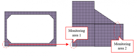
At the entrance of the sharp-curve sections in tunnels, due to sudden changes in cross-section and direction, the pressure fluctuations and velocity changes induced by the fluid generate higher dynamic stress concentrations, reaching maximum values. Similarly, at the exit of the sharp-curve sections, a concentration of stress occurs due to the reduction in fluid velocity and recovery of pressure. In the straight sections of the tunnel, where the pressure distribution of the flow field is relatively uniform and friction loss between the fluid and tunnel walls is minimal, the stress distribution remains relatively stable with minor changes in stress values. However, on the inner side of the sharp-curve sections, due to an increase in flow velocity and a decrease in pressure, stress values significantly increase compared to the outer side. The maximum deformation may occur at the junction between the sharp-curve sections and the straight sections, potentially reaching up to 5.0μm. The deformation distribution throughout the tunnel presents a symmetric pattern centered around the point of maximum deformation, gradually decreasing from the sharp-curve section towards both ends. Figures 2 and 3 provide schematic diagrams of the cross-sectional monitoring area and the layout of monitoring points in the sharp-curve section, respectively.
Figure 2. Schematic diagram of the cross-sectional monitoring area in the sharp-curve section
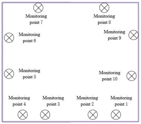
To monitor the dynamic response of the tunnel more thoroughly, especially in critical areas such as the sharp-curve sections, multiple monitoring points can be set up in the simulation model. These monitoring points are located at the entrance, middle, and exit of the sharp-curve sections, as well as at their junctions with straight sections. Particularly at the 45° position of the tunnel, especially on the outer side, a more pronounced response is expected, hence monitoring points can be established in this area to capture the maximum dynamic response. For instance, at the 45° position in the sharp-curve section of the tunnel, three monitoring points might be set: one on the inner wall, one at the top centerline, and another on the outer wall. By comparing data from these monitoring points, it is observed that although the deformation is greatest at the junction of the sharp-curve section, the dynamic response might not be the most intense. Analysis reveals that the location with the greatest dynamic response is at the 45° position on the outer side of the sharp-curve section of the tunnel, thus making the monitoring point at the outer 45° position a focus for further analysis and dynamic simulation calculations.
Figure 3. Layout of monitoring points on the cross-section in the sharp-curve section
2.3 Comparison between steady-state and dynamic simulations
Steady-state simulation considers the mechanical response of tunnel structures when the fluid within the tunnel reaches a stable flow state that does not vary over time. In such cases, while the pressure and velocity of the fluid may be distributed spatially, they remain constant over time. Thus, the stress distribution on the tunnel walls and the deformation of the tunnel structure will also be invariant with time. In sharp-curve tunnel sections, steady flow implies that despite potentially high velocity gradients and pressure differentials within the tunnel, especially at the entrances and exits of sharp curves, these parameters are fixed and do not fluctuate over time. No dynamic disturbances are introduced at monitoring points in steady-state simulations. Similarly, the stress values recorded at stress monitoring points will be constant, showing no fluctuations over time, indicating that under ideal steady-flow conditions, the structural response of sharp-curve tunnel sections is stable, with no accumulation of fatigue risk.
Dynamic simulation, on the other hand, models the variations over time in fluid flow within the tunnel under actual navigation conditions, including non-steady phenomena such as water hammer pressure fluctuations. Under navigation conditions, disturbances caused by the passage of ships and random water flow fluctuations can lead to temporal variations in tunnel internal flow velocity and pressure. When water hammer pressure fluctuations or unsteady flows are present within sharp-curve tunnel sections, the tunnel walls are subjected to non-periodic or periodic mechanical loading. These loadings produce varying stresses on the tunnel structure. In dynamic simulations, monitoring points may record peaks in vibration acceleration, indicating the tunnel's response to changing fluid dynamics under navigation conditions. Likewise, the stress at monitoring points will vary periodically with changes in fluid parameters, reflecting the tunnel's dynamic response to the action of fluid under water hammer pressure fluctuations.
Through comparative analysis of steady-state and dynamic simulations, it is revealed that structural responses of sharp-curve tunnels under navigation conditions exhibit significant differences between dynamic and steady conditions. Under steady conditions, the stress and vibration responses of the tunnel structure may be underestimated, as in actual operational conditions, the tunnel will face unstable changes in pressure and flow velocity caused by ship movement, water flow fluctuations, and other factors.
Conducting global sensitivity analysis and multi-objective optimization studies on the dynamic response parameters of tunnel structures is crucial for ensuring the safety and functionality of tunnels in complex fluid dynamic environments. Through sensitivity analysis, the range of design parameters can be effectively narrowed, focusing resources on more detailed studies to avoid blindness and redundancy in engineering design and construction, thereby enhancing the efficiency and cost-effectiveness of the design. At the same time, multi-objective optimization can balance objectives related to structural safety, construction cost, and operational efficiency, providing a comprehensive optimal solution that considers multiple factors for tunnel design.
In the study of global sensitivity analysis and multi-objective optimization for dynamic response parameters of tunnel structures in sharp-curve sections, a series of structural and response parameters need to be considered. Structural parameters specifically include tunnel wall thickness, tunnel material properties, tunnel cross-sectional shape, burial depth, and overburden characteristics. Response parameters specifically include stress response, displacement response, and fatigue life. During global sensitivity analysis, an assessment is made of which structural parameters have the greatest impact on the tunnel's dynamic response. In the multi-objective optimization process, an attempt is made to find the optimal combination of these parameters to achieve the best balance of the aforementioned optimization objectives.
3.1 Global sensitivity analysis
For a tunnel model containing j parameters, the parameter space for tunnel structure design must first be defined, identifying those key structural parameters that influence the dynamic response of the tunnel. Then, through sampling methods such as Monte Carlo simulation or Latin hypercube sampling, a series of initial parameter vector sets are randomly generated within this parameter space. These vector sets represent possible combinations of tunnel design parameters and will serve as the basic dataset for global sensitivity analysis. Assuming the randomly generated initial vector sets are represented by A=(a1,a2,...,aj), with the number of divisions within the parameter value range space represented by o, the following is obtained:
$\left\{0, \frac{1}{o-1}, \frac{2}{o-1}, \ldots, 1-\Delta\right\}$ (5)
For each parameter, a range of variation is determined. The range of variation can be set based on the importance of the parameter's impact on structural performance with different amounts of variation, or a uniform percentage or fixed amount of variation can be established. After determining the range of variation, each parameter will fluctuate above and below its baseline value to assess the impact of parameter changes on dynamic response. Assuming the set variation is represented by $\Delta$, the value of $\Delta$ can be determined by the following equation:
$\Delta=\frac{1}{o-1}$ (6)
Using the designed experimental scheme, each generated parameter vector set is simulated or calculated, and the dynamic response of the tunnel is recorded. For the response of each parameter vector set, relevant metric data are extracted, which will be used for further analysis of the impact of each parameter. Assuming the system model output response corresponding to the initial parameters is represented by B(A), and the output response produced by the model after the variation Δ of the u-th input parameter is represented by B(a1,...,au-1,au+Δ,...,aj). The following equation provides the calculation formula for the fundamental effect of the u-th input parameter:
$R R_{1 i}=\frac{B\left(a_1, \ldots, a_{u-1}, a_u+\Delta, \ldots, a_j\right)-B(A)}{\Delta}$ (7)
Statistical methods of sensitivity analysis are employed to process the data obtained from simulation or calculation. For each structural parameter, the mean and standard deviation of the corresponding dynamic response metrics are calculated. The mean reflects the average effect of parameter changes, while the standard deviation indicates the fluctuation and uncertainty of parameter changes. The calculations are as follows:
$\omega_u=\sum_{k=1}^v R R_{u k} / v$ (8)
$\delta_u=\sqrt{\sum_{k=1}^v\left(R R_{u k}-\omega_u\right)^2 / v}$ (9)
3.2 Multi-objective optimization
After determining the optimization parameters and objectives for the multi-objective optimization process of tunnel structure, a tunnel model is constructed based on combinations of structural parameters including tunnel wall thickness E, tunnel material characteristics f, tunnel cross-sectional shape parameters α2X, and burial depth and overburden characteristics parameters X. The corresponding stress response, displacement response, and fatigue life serve as surrogate models for the responses.
In FSI issues, the dynamic response of tunnel structures depends on a variety of factors. Initially, a substantial number of data points, including the aforementioned structural parameters and corresponding response parameters, need to be collected or generated. Suppose the structural parameters generated by spatial sample points are represented by A, and the response performance obtained through numerical simulation is represented by B. Assume the u-th structural parameter sample Eu is represented by au=[Eu fu αu Xu], with material characteristics represented by fu, tunnel cross-sectional shape parameters by αu, and burial depth and overburden characteristics parameters by Xu. When structural parameters are au, the response performance of the tunnel structure model is represented by bu. The tunnel structure's stress response is represented by X_WE, displacement response by O, and fatigue life by $\lambda$:
$A=\left[\begin{array}{l}a_1 \\ a_2 \\ a_3 \\ \vdots \\ a_v\end{array}\right]=\left[\begin{array}{cccc}E_1 & f_1 & \alpha_1 & X_1 \\ E_2 & f_2 & \alpha_2 & X_2 \\ E_3 & f_3 & \alpha_3 & X_3 \\ \vdots & \vdots & \vdots & \vdots \\ E_v & f_v & \alpha_v & X_v\end{array}\right]$ (10)
$B=\left[\begin{array}{l}b_1 \\ b_2 \\ b_3 \\ \vdots \\ b_v\end{array}\right]=\left[\begin{array}{ccc}X \_W E\left(a_1\right) & O\left(a_1\right) & \lambda\left(a_1\right) \\ X \_W E\left(a_2\right) & O\left(a_2\right) & \lambda\left(a_2\right) \\ X \_W E\left(a_3\right) & O\left(a_3\right) & \lambda\left(a_3\right) \\ \vdots & \vdots & \vdots \\ X \_W E\left(a_v\right) & O\left(a_v\right) & \lambda\left(a_v\right)\end{array}\right]$ (11)
Utilizing these data points, polynomial regression methods can be applied to fit the relationship between structural parameters and response parameters. Since the response parameters may be affected by random noise, this relationship also needs to incorporate a random process to consider the randomness in the data. This random process is assumed to be a normal distribution with a mean of zero, modeling uncertainty factors. Suppose the polynomial regression function is represented by d(α,m..,au), the random process of zero mean normal distribution by γ(au), vectors composed of o polynomials by d(au), and the regression coefficient vector by α. Thus, the relationship between au and bu can be expressed as a superposition of d(α,m..,au) and $\gamma$(au):
$b_m\left(a_u\right)=d\left(a_u\right)^S \alpha+\gamma_m\left(a_u\right) u=1,2, \ldots, v m=1,2, \ldots, w$ (12)
Suppose the variance of the response process is represented by $\delta^2$, and the correlation coefficient of parameters by $E\left(\phi, a_u, a_k\right)$. The covariance matrix of $\gamma\left(a_u\right)$ is as follows:
$\begin{aligned} & \operatorname{COV}\left[\gamma_m\left(a_u\right), \gamma_m\left(a_k\right)\right]=\delta_m^2 E\left(\varphi, a_u, a_k\right) \\ & u, k=1,2, \ldots, v m=1,2, \ldots, w\end{aligned}$ (13)
Assuming a new set of structural parameters is represented by $a^*$, and the coefficient vector for $v^* 1$ is denoted by $z$. The $m$ columns of the response sample matrix $B$ are represented by $b_m$. The response performance obtained from the numerical model constructed based on $a^*$ can be characterized by a linear combination of the original sample responses:
$\hat{b}_m\left(a^*\right)=z^S b_m m=1,2, \ldots, w$ (14)
Thus, the prediction error is given by:
$\begin{aligned} & \hat{b}_m^*\left(a^*\right)-b_m^*\left(a^*\right)=z^S b_m-b_m\left(a^*\right) \\ = & c^T Z_l-c_m\left(a^*\right)+\left(D^S z-f\left(a^*\right)\right)^S \alpha_m\end{aligned}$ (15)
where,
$C_m=\left[c_1\left(a_1\right), c_1\left(a_2\right), \ldots, c_1\left(a_v\right)\right]$ (16)
$D=\left[\begin{array}{ccc}d_1\left(a_1\right) & \cdots & d_o\left(a_1\right) \\ \vdots & \ddots & \vdots \\ d_1\left(a_v\right) & \cdots & d_o\left(a_v\right)\end{array}\right]$ (17)
Setting the mean of the prediction error to zero yields:
$D^S z-d\left(a^*\right)=0$ (18)
The Kriging model, serving as a surrogate model, plays a central role in this process. It employs the EXP correlation function to describe the spatial correlation between different data points. The following equation provides the calculation formula for the mean square error prediction of the Kriging surrogate model:
$\begin{gathered}\psi_m\left(a^*\right)=R\left[\left(b_m^*\left(a^*\right)-b_m\left(a^*\right)\right)^2\right] \\ =R\left[\left(z^S c_m-c_m\left(a^*\right)\right)^2\right]=\delta_m^2\left(1+z^S E z-2\right)\end{gathered}$ (19)
The introduction of Lagrange multipliers ensures the calculation of the minimum numerical value for the above equation:
$M(z, \eta)=\delta_m^2\left(1+z^S E z-2 z^S e\right)-\eta^S\left(D^S z-d\left(a^*\right)\right)$ (20)
Deriving z yields:
$M_z^{\prime}(z, \eta)=2 \delta_m^2(E z-e)-D \eta$ (21)
The coefficient vector for the linear combination of responses is solved using the first-order optimality condition, thereby determining the optimal vector of parameter weights and Z:
$z=E^{-1}\left(e-D\left(D^S E^{-1} D\right)^{-1}\left(D^S E^{-1} e-d\left(a^*\right)\right)\right)$ (22)
Any tunnel structure parameter represented by $a^*$, and its target response value represented by $b^*\left(a^*\right)$, is given by:
$b_m^*\left(a^*\right)=E^{-S}\left(e-D\left(D^S E^{-1} D\right)^{-1}\left(D^S E^{-1} e-d\left(a^*\right)\right)\right)^{b S} b_m$ (23)
Upon obtaining the results of numerical simulations, the response parameters for the new combination of structural parameters can be represented as a linear combination of the original numerical simulation sample response parameters. This step is based on the internal working principle of the Kriging model. The Kriging model does more than merely interpolate; it balances the spatial relationships between sample points and the uncertainty at each point, thus making predictions about unknown points. The coefficients of this linear combination, obtained through model training, can be seen as a mapping from known data points to new data points. In FSI analysis, this means that the dynamic response of the tunnel under new structural parameter configurations can be predicted using existing numerical simulation data, without the need for new, time-consuming simulations.
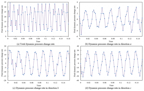
Figure 4 presents the time-domain curves of the rate of change in dynamic pressure at monitoring points within a sharp-curve tunnel under navigation conditions, subjected to the action of water hammer pressure. From the figure, it is observed that under the influence of water hammer pressure, the fluctuation amplitude of the rate of change in dynamic pressure at monitoring points in different directions (c and b directions) is significantly larger, while in the a direction, the fluctuation amplitude is smaller. Although the fluctuation amplitudes differ across directions, the phase of the rate of change in dynamic pressure remains consistent due to the unchanging frequency of water hammer pressure fluctuations. Based on the observed phase consistency, it can be inferred that the pulsation frequency of the total dynamic pressure change rate at the monitoring points is twice as high in all directions. These results indicate that despite the differences in dynamic pressure change amplitude across directions, the frequency remains consistent, which is attributed to the varying impacts of tunnel geometry, fluid velocity distribution, and tunnel wall resistance distribution in different directions.
It can be concluded that the larger amplitude of dynamic pressure changes in the c and b directions is related to their orientation relative to the fluid's main flow direction or the tunnel wall's relative position. The curvature of the tunnel results in an uneven distribution of velocity gradients in different directions, leading to variations in the amplitude of dynamic pressure changes across directions. The frequency of fluctuations produced by water hammer pressure is associated with the regularity of ship passages, such as the speed, size, and interval of ships passing through, which causes the frequency of dynamic pressure changes to remain consistent across all directions. Since the fluctuation frequency and phase are the same in all directions, the total rate of change in dynamic pressure appears as a superposition of these frequencies. The pulsation of the total dynamic pressure change rate reflects a higher frequency due to the superposition of vibrations in all directions. If the phase and frequency of dynamic pressure change rates in all directions remain unchanged, the inference of the pulsation frequency doubling requires further verification. Typically, a doubling of frequency implies the presence of nonlinear effects or interaction mechanisms, stemming from complex interactions between the tunnel structure's inherent vibration modes and the action of fluid dynamics.
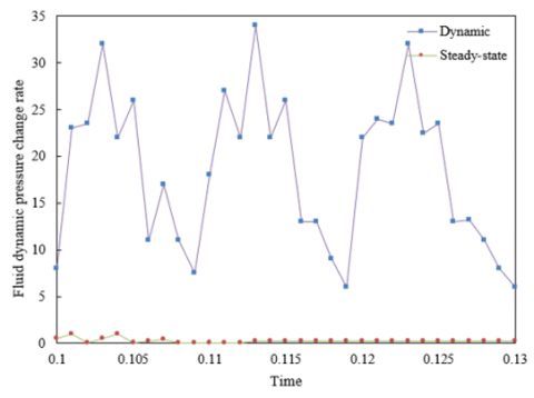
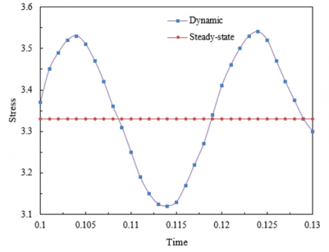
Figures 5 and 6 provide a comparison between the dynamic and steady-state fluid dynamic pressure change rates and stress at monitoring points in the sharp-curve tunnel section. From these figures, it is evident that when fluid reaches a steady flow within the sharp-curve tunnel, the rate of change in dynamic pressure and structural stress at monitoring points hardly varies over time. This indicates that under steady-state conditions, the fluid flow within the tunnel becomes predictable and stable, and the fluid forces acting on the tunnel structure reach a constant state. In such cases, the design of the tunnel structure can be optimized based on these stable loading conditions. In contrast to steady-state flow conditions, when considering the flow under the action of water hammer pressure, the rate of change in dynamic pressure and stress at monitoring points exhibits periodic variations. Water hammer phenomena typically occur when fluid parameters change suddenly, such as pressure fluctuations caused by ships passing rapidly through the tunnel. These periodic changes indicate that the tunnel structure must be capable of withstanding periodic loads generated by fluid dynamics.
Figure 4. Fluid dynamic pressure change rate (time variation curve)
Figure 5. Comparison of dynamic and steady-state fluid dynamic pressure change rates at monitoring points in the sharp-curve tunnel section
Figure 6. Comparison of stress at dynamic and steady-state monitoring points in the sharp-curve tunnel section
It can be concluded that both steady-state and dynamic flow conditions should be considered in tunnel design. Steady-state flow provides a baseline for static loads, while dynamic flow conditions impose additional requirements on the tunnel's fatigue life and dynamic response characteristics. The FSI effects are particularly significant under dynamic flow conditions. The dynamic response of the tunnel is significantly affected by the water hammer effect, necessitating detailed consideration in numerical simulations to predict the structure's dynamic behavior. Monitoring fluid dynamic pressure and structural stress during tunnel operation is crucial for safety assessment and maintenance. Especially for sharp-curve tunnels, due to the complexity of fluid dynamics, continuous monitoring can help prevent structural failures.
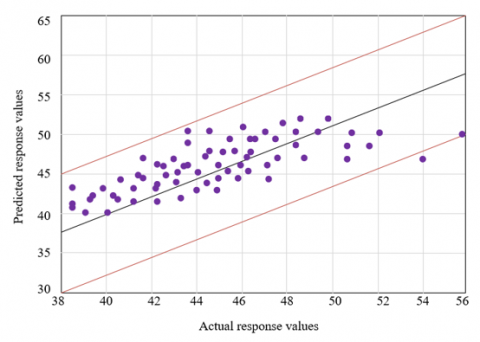
Metamodel of Optimal (MOP), commonly used in systems engineering as a surrogate model, is employed to approximate complex physical models, thereby reducing computational costs. In this study, the MOP was utilized prior to sensitivity analysis to predict the dynamic response of tunnel structures. Figure 7 illustrates the predicted distribution of response values for dynamic response parameters of the sharp-curve tunnel structure. The experimental results show that the actual response values are closely distributed around the prediction curve, indicating high accuracy of the model predictions. Within the OptiSLang software, the Coefficient of Prognosis (COP) serves as an indicator to describe the model fitting accuracy. The range of the COP is from 0% to 100%, where 100% indicates a perfect fit. With a COP of 84%, this high value suggests that the model can reflect actual conditions with high accuracy, and thus, the model's predictions can be considered reliable.
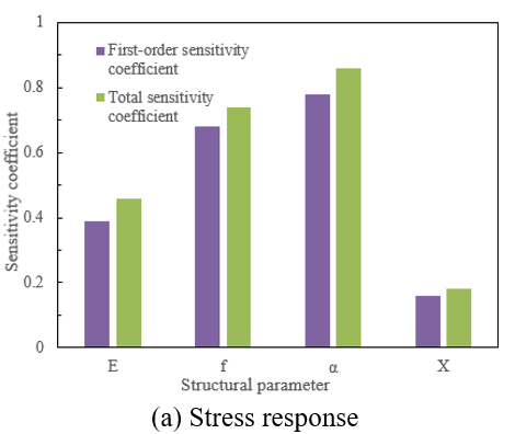
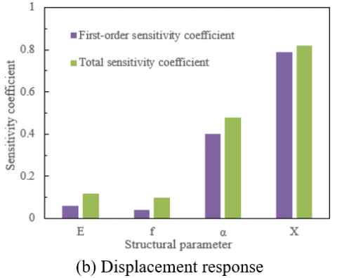
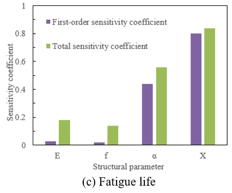
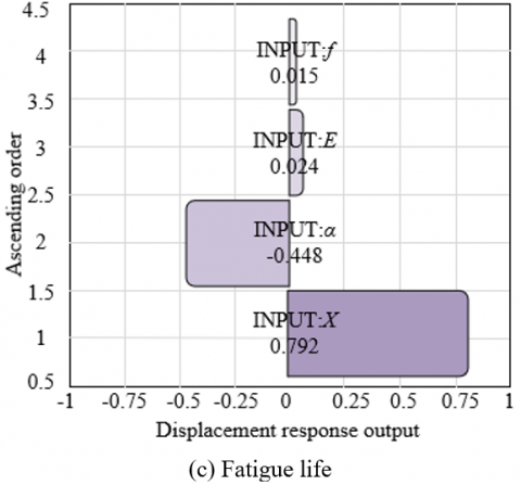
Figure 8 conducts a sensitivity analysis of various structural parameters under target responses for the sharp-curve tunnel structure. The experimental results provide an analysis of the sensitivity results of structural parameters under each target response in the sharp-curve tunnel. In the sensitivity analysis results for the sharp-curve tunnel, the structural parameters are tunnel wall thickness E, tunnel material characteristics f, tunnel cross-sectional shape parameter α, and burial depth and overburden characteristics parameter X. Figure 8(a) represents the stress response indicator, showing the impact of changes in four structural parameters on the stress response of the sharp-curve tunnel structure. It is found that the sensitivity coefficient of the tunnel cross-sectional shape parameter is the largest, indicating that its variation has the greatest impact on stress response. The impact of tunnel material characteristic parameters on stress response is second only to that of the cross-sectional shape parameter. The impact of tunnel wall thickness and burial depth, overburden characteristics parameters on the stress response of the sharp-curve tunnel structure is minor, with the impact of burial depth, overburden characteristics parameters on stress response being negligible. With displacement response and fatigue life as response indicators, the impact of changes in four structural parameters on them is shown in Figures 8(b) and (c). It is observed that the sensitivity analysis results for displacement response, fatigue life predominantly share great similarity, with the changes in burial depth, overburden characteristics parameters having the greatest impact, followed by the impact of tunnel cross-sectional shape parameters; the impact of tunnel wall thickness and tunnel material characteristics is the least.
Based on the above analysis results, the following inferences and conclusions can be drawn: In designing sharp-curve tunnels, special attention should be paid to the design of the tunnel cross-sectional shape, as it is the most sensitive to stress response. Choosing an appropriate cross-sectional shape can significantly improve the structural safety of the tunnel. Tunnel material characteristics are also critical in design, closely following the tunnel cross-sectional shape in terms of impact on stress response. Therefore, in selecting materials, both their performance and cost should be considered to achieve a balance between economy and safety. The burial depth and overburden characteristics become particularly important when considering the tunnel's stability and displacement resistance. Therefore, geological surveys and analysis work should be emphasized in the planning and design stages to reduce potential geological risks in the future. Although the impact of tunnel wall thickness on stress response is smaller, its synergistic effects with other structural parameters still need to be properly considered to ensure optimization of the design.
Figure 7. Predicted distribution of response values for dynamic response parameters of the sharp-curve tunnel structure
Figure 8. Sensitivity analysis of structural parameters under target responses
Figure 9. Correlation analysis of various structural parameters under target responses
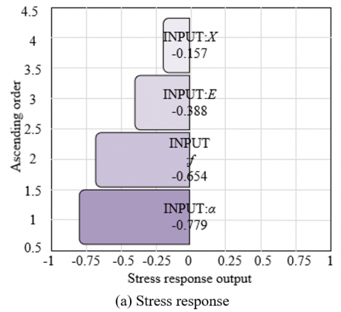
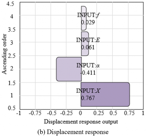
The analysis of the correlation between various structural parameters under target responses for the sharp-curve tunnel, as shown in Figure 9, indicates that the degree of impact of each parameter on the structural stress response indicator, in descending order, is: tunnel cross-sectional shape parameter, tunnel material characteristics, tunnel wall thickness, and burial depth and overburden characteristics parameters. For indicators of displacement response and fatigue life, the degree of impact of each parameter, in descending order, is: burial depth and overburden characteristics parameters, tunnel cross-sectional shape parameter, tunnel wall thickness, and tunnel material characteristics, which is largely consistent with the sensitivity analysis results presented in Figure 8.
It can be concluded that for displacement response and fatigue life, these parameters play the most crucial role. The physical characteristics of the burial depth and overburden, such as density and elastic modulus, affect the magnitude and distribution of tunnel displacement, and also determine the tunnel's fatigue behavior under long-term load actions. Next is the tunnel's cross-sectional shape, which also plays an important role in displacement response and fatigue life. An appropriate cross-sectional shape can offer better stability and resistance to deformation. As for tunnel wall thickness and material characteristics, their impact on displacement response and fatigue life is less significant than the former two but remains parameters worthy of attention. Especially in considering fatigue life, the durability of the material and sufficient wall thickness can reduce the formation of cracks and extend the tunnel's service life.
The research content and experimental results of this study have been thoroughly discussed and analyzed around two core parts: the study of the FSI effects and the optimization of structural parameters based on global sensitivity analysis. Initially, advanced numerical simulation technology was employed to establish a FSI model for sharp-curve tunnels. The impact of fluid on tunnel structures under navigation conditions was deeply analyzed through the computation of coupled fields of fluid dynamics and structural mechanics. The study revealed the dynamic response of tunnels under the action of fluid, with particular attention paid to the fluid dynamic pressure changes in sharp-curve sections, which is crucial for understanding the performance of tunnels under actual operating conditions. A comparison of fluid dynamic pressure change rates and stress distribution at monitoring points in sharp-curve tunnels under dynamic and steady-state flow conditions provided experimental data support for understanding the stability and safety of tunnel structures under fluid action.
Through global sensitivity analysis, this study revealed the sensitivity of tunnel structural design parameters to dynamic responses, identifying parameters that have the greatest impact on the overall performance of the tunnel. Coupled with sensitivity analysis, a correlation analysis was conducted to understand the interactions between different structural parameters, which is crucial for parameter optimization. Based on the analyses above, multi-objective optimization theory was applied to optimize the structural design parameters of the tunnel. The goal is to enhance economic benefits while ensuring structural safety.
The study of the FSI effect has proven the importance of considering fluid action in the tunnel design process, especially in the design of sharp-curve tunnels where the impact of fluid dynamics is particularly significant. Sensitivity analysis of structural parameters provides targeted guidance for tunnel design. For instance, cross-sectional shape and material characteristics are key parameters affecting stress response, while burial depth and overburden characteristics significantly impact displacement response and fatigue life. The results of multi-objective optimization indicate that by adjusting sensitive parameters, the economic efficiency of tunnel design can be improved without sacrificing safety. This demonstrates that a more optimal design solution can be achieved in the tunnel design process by comprehensively considering structural responses and economic factors.
The research conducted in this study not only provides theoretical basis and methodological guidance for the design of sharp-curve tunnels but also has practical significance for actual engineering projects, assisting engineers in making more scientifically sound decisions during the design and construction process.
This paper was supported by Scientific and Technological Research Program of Chongqing Municipal Education Commission (Grant No.: KJQN201903806) and Scientific and Technological Research Program of Chongqing Municipal Education Commission (Grant No.: KJQN202203808).
[1] Zhang, D., Yang, B. (2023). Construction technology of tunnel lining vault embedded pipe timely grouting. In International Conference on Advances in Civil and Ecological Engineering Research, Macau, China, pp. 112-121. https://doi.org/10.1007/978-981-99-5716-3_9
[2] Islam, A., Abdullah, R.A., Ibrahim, I.S., et al. (2023). Effect of stress ratio k due to varying overburden topography on crack intensity of tunnel liner. Journal of Performance of Constructed Facilities, 37(4): 04023026. https://doi.org/10.1061/JPCFEV.CFENG-4281
[3] Wang, D., Chen, C., Zhang, H., Liu, Z., Meng, S. (2023). Influence of gas explosion in a utility tunnel on the structural safety of an undercrossing tunnel. Zhendong yu Chongji/Journal of Vibration and Shock, 42(8): 160-166 and 185.
[4] Zheng, H., Li, P., Ma, G., Zhang, Q. (2022). Experimental investigation of mechanical characteristics for linings of twins tunnels with asymmetric cross-section. Tunnelling and Underground Space Technology, 119: 104209. https://doi.org/10.1016/j.tust.2021.104209
[5] Fu, Y.B., Mei, C., Bian, Y.W., Zhang, X.L., Wang, F.D., Hu, Y. (2022). Analytical solution and application of large-diameter shield segment uplift considering the filling rate of grouting. Zhongguo Gonglu Xuebao/China Journal of Highway and Transport, 35(11): 171-179.
[6] Chen, Q., Zhang, T., Hong, N., Huang, B. (2021). Seismic performance of a subway station-tunnel junction structure: A shaking table investigation and numerical analysis. KSCE Journal of Civil Engineering, 25: 1653-1669. https://doi.org/10.1007/s12205-021-1169-4
[7] Yu, H., Zhang, Z., Chen, J., Bobet, A., Zhao, M., Yuan, Y. (2018). Analytical solution for longitudinal seismic response of tunnel liners with sharp stiffness transition. Tunnelling and Underground Space Technology, 77: 103-114. https://doi.org/10.1016/j.tust.2018.04.001
[8] Kundanati, L., Chahare, N.R., Jaddivada, S., Karkisaval, A.G., Sridhar, R., Pugno, N.M., Gundiah, N. (2020). Cutting mechanics of wood by beetle larval mandibles. Journal of the Mechanical Behavior of Biomedical Materials, 112: 104027. https://doi.org/10.1016/j.jmbbm.2020.104027
[9] Liu, J.Y., Xia, C.C. (2011). Research on computing method of similarity scale of dynamic model test concerning fluid-structure coupling for water-conveyance tunnel. Applied Mechanics and Materials, 80: 626-630. https://doi.org/10.4028/www.scientific.net/AMM.80-81.626
[10] Liu, J.Y., Chen, J.Y. (2008). A similarity technique for water-conveyance tunnel dynamic model test considering fluid-structure coupling. Yantu Lixue/Rock and Soil Mechanics, 29(12): 3387-3392.
[11] Chen, J.Y., Liu, J.Y. (2006). Fluid-structure coupling analysis of water-conveyance tunnel subjected to seismic excitation. Yantu Lixue/Rock and Soil Mechanics, 27(7): 1077-1081.
[12] Cao, L., Yang, P.F., Wang, Y.X., Chen, G. (2019). Wind tunnel experimental study on noise of flexible thin plate wing with fluid-solid interaction effects. Zhongguo Kexue Jishu Kexue/Scientia Sinica Technologica, 49(7): 815-824.
[13] Ivanco, T.G., Keller, D.F., Pinkerton, J.L. (2020). Investigation of atmospheric boundary-layer effects on launch-vehicle ground wind loads. In 2020 IEEE Aerospace Conference, Big Sky, MT, USA, pp. 1-20. https://doi.org/10.1109/AERO47225.2020.9172608
[14] Wang, W., Zhou, L., Wang, Z., Escaler, X., De La Torre, O. (2019). Numerical investigation into the influence on hydrofoil vibrations of water tunnel test section acoustic modes. Journal of Vibration and Acoustics, 141(5): 051015. https://doi.org/10.1115/1.4043944
[15] Guo, Y.M., Yan, J.G., Xing, X.J., Wu, C.H., Chen, X.R., Li, F.H. (2020). Modeling and analysis of deformed parafoil recovery system. Xibei Gongye Daxue Xuebao/Journal of Northwestern Polytechnical University, 38(5): 952-958.
[16] Zhang, J., Tan, C.X., Xu, K.C. (2021). Nonlinear dynamic response analyses of a soft soil-tunnel-aboveground frame structure system under earthquake. Zhendong yu Chongji/Journal of Vibration and Shock, 40(12): 159-167.
[17] Guan, X.M., Nie, Q.K., Li, H.W., An, J.Y. (2019). Research overview on dynamic response and damage of existing structure under tunnel blasting vibration. Tumu Gongcheng Xuebao/China Civil Engineering Journal, 52: 151-158.