Nibal Fadel Alhialy![]()
© 2023 IIETA. This article is published by IIETA and is licensed under the CC BY 4.0 license (http://creativecommons.org/licenses/by/4.0/).
OPEN ACCESS
In the field of nuclear reactor design, precise calculation of reactor dimensions is crucial for operational efficiency and safety. This study focuses on the critical dimension prediction for a spherical nuclear thermal reactor, employing a computational approach to address this challenge. Utilizing the two-group neutron diffusion equation, the research aims to establish a mathematical model for neutron distribution within the reactor's geometry. A key aspect of this model involves the prediction of neutrons' spatial distribution, essential for understanding the reactor's behavior under operational conditions. The methodology adopted in this investigation involves using a MATLAB-based program specifically developed for solving the two-group diffusion equation in spherical reactor geometry. This approach facilitates the determination of exact dimensions and optimal fuel mass for the reactor. The study's findings indicate a critical core radius of 21.7 cm, with a water mass of 40.5 kg and a U235 fuel mass of 1.12 kg. Additionally, the ratio of fast flux to slow flux was approximately 1.5. These results not only align closely with prior research in this domain but also enhance the understanding of spherical reactor design. Crucially, the study's outcomes demonstrate a high degree of compatibility with existing literature, thereby reinforcing the validity of the computational model used. This research contributes significantly to the nuclear engineering field by providing a robust method for determining the critical dimensions and mass of fuel required for the efficient and safe operation of spherical nuclear thermal reactors. Which still regarded nuclear energy as an essential partner in friendly energy production in the world to reduce CO2 emissions. The implications of these findings are substantial, offering a pathway to optimized reactor design and a deeper understanding of neutron behavior in complex geometrical configurations.
neutron diffusion equation, neutron transport theory, critical mass, nuclear energy, nuclear spherical core size, PWR, sustaining chain reaction, CO2 emissions
In the context of an increasing global demand for sustainable and environmentally friendly energy solutions, nuclear energy has garnered significant attention due to its potential to meet a substantial portion of the world's energy needs. This attribute positions nuclear power as a leading energy source. It has been documented that, with regular maintenance, nuclear plants can operate over extended periods with minimal fuel consumption, thereby offering a more efficient alternative compared to other energy sources [1]. The World Nuclear Association (WNA) has set a target for nuclear energy to provide 25% of global electricity by 2050. Achieving this goal necessitates the construction of new nuclear power plants, cumulatively contributing approximately 1000 GWatt in electrical capacity. This expansion underscores the importance of optimizing safety and performance, considering various factors such as reactor lifecycles and increasing electricity demands, and decreasing CO2 release [2].
The construction of nuclear reactors is a task of profound environmental and economic significance. During operation, the primary goal is to sustain a chain reaction, maintaining a balance between the neutrons produced by fission and those consumed or lost from the reactor. This balance is crucial for the reactor’s efficiency and safety. Research in nuclear energy has traditionally been divided between neutron transport theory studies and dynamic kinetic model research [3]. These studies encompass the dynamic behaviors of nuclear reactors, including the temporal variation of power release and the delayed release from decayed power sources. The power output of a reactor consists of immediate energy from fission reactions and the energy from the decay of fission fragments.
Additionally, the nuclear calculation involves investigations into the dynamic transient performance of the pressurizer in nuclear pressurized water reactors (PWR) [4-6]. The pressurizer's behavior has been modeled using differential equations and genetic algorithms, and these models have been compared to understand their efficacy. Furthermore, comprehensive reviews have been conducted on the studies and revisions related to the pressurizer system. These encompass theoretical modeling, experimentation, and transient operation tests, which are essential for controlling the design parameters of nuclear reactors.
The structure of a reactor, defined by its geometry and material composition, dictates the chain reaction's regulation. This control is often achieved through the insertion or removal of control rods. The application of neutron transport theory is essential, as it describes the mechanism for generating heat in a safe, controlled manner through a stable and continuous fission reaction. The high cost associated with building a nuclear reactor is primarily due to the necessity for precise neutron transport modeling. Addressing these challenges is imperative for designing nuclear power stations that ensure the security and safety of the reactor.
The objective of this research is to derive and solve the two-group diffusion equation for a spherical geometry reflected thermal reactor. The study employs MATLAB to simulate the mathematical equation, focusing on the arrangement techniques for the two-group diffusion equation. This approach offers a feasible approximation for estimating and designing nuclear reactors. Additionally, the research presents an analytic mathematical model for the two-group neutron diffusion equation, aimed at determining critical reactor dimensions such as nuclear radius, fuel, and moderator mass, as well as elucidating the neutron flux distribution in a spherical critical nuclear reactor.
Historically, the discovery in 1938 that a neutron can split uranium, releasing substantial energy, marked a significant advancement in nuclear science. The identification of the uranium-235(U235) isotope and its ability to undergo fission while releasing additional neutrons, initiated the concept of a sustained chain reaction for energy production [7].
In nuclear thermal reactor descriptions, a minimum of two neutron groups is typically considered. The first group, referred to as fast neutrons, possesses energy levels exceeding those of thermal neutrons. Conversely, the second group, or the two-group neutrons, exclusively comprises thermal neutrons, which have transitioned from the fast energy region to the thermal energy region. For accurate and realistic criticality calculations in thermal reactors, the employment of two-group neutron models is essential. The two-group neutron diffusion equations can be resolved through either analytical or numerical methods. When approached analytically, the boundary conditions of group-diffusion theory pertain to the neutron flux in relation to the normal current at the core-reflector interfaces, taking into account the reflector's specific constraints [8].
The spherical thermal core, with a radius denoted as R, incorporates a reflector of a specified depth [9]. This is a critical factor in determining the size of the reactor core. The core and reflector of the reactor are analyzed using a four-group diffusion equation, integral to the criticality calculation. This approach involves solving core neutron fluxes through eight linearly independent functions. A noteworthy correspondence was observed between the analytical results derived from the diffusion code, ALBD4G, and the discretized solutions obtained from code citation calculations of the Keff value. This comparison revealed a minimal error margin, approximately 0.3%, underscoring the precision of the analytical method employed.
Hosseini [10] developed an innovative three-dimensional (3D) computational code employing the Galerkin finite element method (GFEM). This code was specifically designed to solve multi-group forward/adjoint diffusion equations applicable to various geometrical configurations, including hexagonal and quadrangular shapes.
Shqair et al. [11] presented a comprehensive study on multi-energy groups of neutron diffusion equations, which were analytically solved using the power series method. This study encompassed an examination of three distinct geometrical forms: slab, cylinder, and sphere. The general solution addressed both the two-group diffusion and encompassed four energy groups of neutrons. This analytical process involved a series of numerical calculations, conducted within predetermined limit conditions, resulting in the production of an analytical flux. Significantly, the flux associated with these multi-energized groups in the theory of neutron diffusion exhibited a radial distribution. Consequently, the dimensions of the reactor core, crucial in the context of criticality, were specified using the variable µ.
In terms of reflected reactors, Shqair and El-Zahar [12] successfully obtained an analytical solution for the neutron diffusion equation using the method of differential transform modification (MDTM). This method involved the precise application of MDTM to address initial value problems, both particular and non-particular, that are crucial for various reactor geometries. The application of MDTM was specifically focused on reactors comprising both core and reflected components, akin to bare reactors, which include the fuel core. The effectiveness and reliability of this method were confirmed through its ability to accurately solve such complex cases, thereby contributing significantly to the field of nuclear reactor analysis.
In conclusion, the determination of a reactor's geometrical core shape, size, and materials necessitates consideration of the nuclear fuel to moderator mass ratio. This aspect is vital for ensuring the safe and reliable operation of nuclear reactors, particularly in cross-section calculations where precision is paramount, as evidenced in the nuclear industry's preference for single-digit separators in such measurements.
The methods used for the calculation of the nuclear reactor design are very complex because, for any nuclear chain reaction system, the modeling of the growth of neutrons is complicated because of the continuous variation in energy and direction. This variation complexly affects cross-sections. This difficulty is increased by the emission of secondary neutrons.
First, we made these assumptions:
There is no interesting source of neutrons in the medium.
Homogeneous medium, that is, independent of three-dimensional location for neutron cross-section.
Isotropic distribution of neutrons with angular pattern at the medium.
Approximately uniform flux at the medium.
Infinite consideration medium [13].
Neutrons produced from a fissionable material source can be lost by absorption in different reactions with nuclei or by leakage from the volume element. The net changing rate is the density of the neutron, n, at any time, t, and a point in V, with time, $\frac{\partial n}{\partial t}$ will be:
$\int_{\mathrm{V}} \frac{\partial \mathrm{n}}{\partial \mathrm{d}} \mathrm{dV}=\int_{\mathrm{V}} S \mathrm{~d} V-\int_{\mathrm{V}} \sum_{\mathrm{a}} \varnothing \mathrm{dV}-\int_{\mathrm{V}} \operatorname{div} \mathrm{J} \cdot \mathrm{dV}$ (1)
where,
$\int_V \frac{\partial n}{\partial t} d V$=Neutron density Change Rate,
$\int_V S d V$=NeutronProduction Rate,
$\int_{\mathrm{V}} \sum_{\mathrm{a}} \emptyset \mathrm{dV}$=Absorption Rate,
$\int_{\mathrm{V}} \operatorname{div} \mathrm{J} \cdot \mathrm{dV}$=Leakage Rate,
The source strength of neutrons is the neutron numbers emitted per second/unit volume, and J is the current of the neutrons.
The establishment of the equation of continuity is done by merging the previous equations into Eq. (1). One must compute all of the above integrals over the same terminated volume, such that the summation of integrals on the right is equal to the summation of integrals on the left. Therefore,
$\frac{\partial \mathrm{n}}{\partial \mathrm{t}}=\mathrm{S}-\sum_{\mathrm{a}} \emptyset-\operatorname{div} \mathrm{J}$ (2)
For a steady state (that is not dependent on time (and from the current definition, the meaning of flux is connected by the law of Fick's scientist $(\mathrm{J}=-\mathrm{D} \nabla \emptyset)$:
$\mathrm{D} \nabla^2 \emptyset-\sum_{\mathrm{a}} \emptyset+\mathrm{S}=$ (3)
Dividing by D,
$\nabla^2 \emptyset-\frac{1}{\mathrm{L}^2} \emptyset=-\frac{\mathrm{s}}{\mathrm{D}}$ (3')
where, $\frac{\sum_{\mathrm{a}}}{\mathrm{D}}=\mathrm{L}^2$ is called the diffusion area.
This is the steady-state one-group diffusion equation, where $\nabla^2$ is called the Laplacian, which is different according to the shape of the reactor, as also for spherical geometry:
$\nabla^2=\frac{1}{\mathrm{r}^2} \frac{\partial}{\partial \mathrm{r}} \mathrm{r}^2 \frac{\partial^2 \emptyset}{\partial \theta}$.
Then to solve the second-order equation, the boundary conditions must be determined, because the critical radius R is the dimension of the reactor that is determined as the flux vanishes. The general boundary conditions are:
The flux of neutrons must be limited, and non-negative in all regions in which the diffusion equation is satisfied.
Boundary Conditions of Symmetry: This means the current at the interface = zero.
$\mathrm{d}=0.71 \lambda_{\mathrm{tr}}=$ transport mean free path $=3 \mathrm{D}$.
Vacuum Boundary Condition: Such boundaries are approximated utilizing flux = zero.
Interface Boundary Condition for different media:
$\emptyset_{\mathrm{A}}=\mathrm{J}_{\mathrm{A}}=\mathrm{J}_{\mathrm{B}}$
A homogeneous mixture of an infinite spherical reactor consists of a fuel material and a moderator material, with low fuel concentration. The one-velocity reflected reactor is internally assumed as a homogeneous multiplying medium, the flux is a function of (r) only the core, see Figure 1.
The aim is to determine the critical radius, critical mass, and thermal flux distributions of a one-watt power homogeneous spherical thermal reactor at room temperature. The reactor is fueled with U235 and moderated as well as reflected by ordinary water. One can assume the reactor to have an infinite water reflector. An infinite reflector is one whose thickness is much larger than both the slowing down and diffusion lengths in the reflector. Practically all reactors have reflectors of infinite type. The ratio of atoms of U235 to molecules of water in the core equaled to be $\left[\frac{\mathrm{N}_{235}}{\mathrm{~N}_{\mathrm{W}}}=\frac{1}{500}\right]$ [14].
Neutron current density (n), neutron flux (Ø), neutron current (J), and coefficient of diffusion (D) variables are associated. For getting the relation, the derivation of diffusion coefficients depends on the characteristics of the nuclear medium [13].
Neutron current density (n), neutron flux (Ø), neutron current (J), and coefficient of diffusion (D) variables are associated. For getting the relation, the derivation of diffusion coefficients depends on the characteristics of the nuclear medium [13].
Figure 1. Diagram of the spherical reactor, with reflector
4.1 Two group model
The one-group method did not fully consider the size of criticality or structure of a thermal reactor. As most of the thermal neutrons are generated from the energy of slowing neutrons through diffusion to a specific distance, it should be considered that this fast neutron in a designed nuclear reactor. Any design process of a thermal nuclear reactor must obviously be represented by two neutron groups at least. Fast neutrons are the first group, with energies above the thermal region, and the second group is the thermal neutrons. In various reactor computations, particularly those including the criticality of thermal reactors, no less than two groups of neutrons must be utilized, to get sensibly precise outcomes. One group is important to depict the thermal neutrons. The second or fast group includes all the neutrons having energies above the thermal - that is, the neutrons that are reducing their energies from fissional energies to thermal energy. Figure 2 shows, schematically, the difference between one- and two-group models. The boundary between these two groups is set to 1 eV [14]. Using the two-group neutron diffusion equation.
By definition, the multiplication constant is (k∞=η ε f p PFNL PTNL). The previous formula is named the six-factor formula. (η), and represents the number of neutrons absorbed in the fuel in the second generation, generated per neutron (ε). This is called the fast fission factor and is the amplification in the number of fast neutrons due to fast fissions. (P), called the resonance escape probability, is the fraction of fast neutrons that succeed in slowing down. Finally, (f) is defined as the thermal-utilization factor. It represents the percent of neutrons absorbed by the fuel. PFNL is the probability that a fast neutron will not leak out of the system. (PTNL), is the probability that a thermal neutron will not leak out of the system.
Figure 2. Life cycle of thermal neutrons both in (a) the one-group model and (b) the two-group model
4.2 Core
The two-group model assumes that the represented equation in each region (core+reflector) is a single exact diffusion equation involving the fast-neutron cross-sections, which can represent the fast neutron response in a reactor with a reflector. The number of neutrons lost from the fast group per unit volume, per second, is the slowing down into the thermal group. Further, it is the slowing down of neutrons outside the fast group at any space, which is proportional to the fast-neutron flux ($\emptyset_1$) at that point, thermal flux $\left(\emptyset_t\right)=\left(\emptyset_2\right)$.
Primarily, the equation of diffusion is considered for neutrons with two energy ranges (fast and thermal) in the core, Figure 3. The flux is dependent on one singular spatial inconstant, which (r) is, and a steady state.
To begin with, the energy spectrum is divided into two levels (demonstrated in Figure 3), and then the average macroscopic cross-section has to be computed to be known.
Figure 3. Neutron energy groups
First, we will apply Eq. (3) for the fast neutron group, which is symbolized by a subscript (1). For the thermal neutron group, the variables are denoted by a subscript (2). Then Eq. (3) will be as follows, for a fast group:
$\mathrm{D}_1 \nabla^2 \emptyset_1-\sum_{1 \mathrm{~s}} \emptyset_1-\sum_{1 \mathrm{a}} \emptyset_1+v \sum_{1 \mathrm{f}} \emptyset_1+v \sum_{2 \mathrm{f}} \emptyset_2=0$. (4)
where,
$\sum_{1 \mathrm{~s}} \emptyset_1$: Neutrons slowed downcast proportion inside the thermal -group outside the fast- group, per cm3/sec, thermal-neutrons producer.
$\sum_{2 \mathrm{a}} \emptyset_1$: slowing group-absorbing rate of the fuel-moderator mixture.
$\sum_{1 f}$: Fast and thermal fission rates respectively.
v: The mean neutrons number generated per fission at the medium (2.43 for U235), & Eq. (3) will be as follows for the thermal group:
$\mathrm{D}_2 \nabla^2 \emptyset_2-\sum_{2 \mathrm{a}} \emptyset_2+\sum_{1 \mathrm{~s}} \emptyset_1=0$ (5)
In a thermal reactor, the neutrons appear in the fast group as the result of fissions induced by thermal neutrons. There are no fissions caused by fast neutrons, as only neutrons absorbed in the thermal group produce fast neutrons. Neutrons are lost from the fast group when slowing down. We will denote core reflector regions as, one (1c, 1r) for the fast group and (2c, 2r) for the thermal group; Eqs. (4) and (5) will be:
$\mathrm{D}_{1 \mathrm{C}} \nabla^2 \emptyset_{1 \mathrm{C}}-\sum_{1 \mathrm{Cs}} \emptyset_{1 \mathrm{C}}+\frac{\mathrm{K}_{\infty}}{\mathrm{P}_{\mathrm{C}}} \sum_{2 \mathrm{Ca}} \emptyset_{2 \mathrm{C}}=0$ (6)
$D_{2 C} \nabla^2 \emptyset_{2 C}-\sum_{2 C a} \emptyset_{2 C}+P_C \sum_{1 C s} \emptyset_{1 C}=0$ (7)
where, PC: leaves the neutrons fraction in the fast group, it enters the thermal group in the core [15].
In both groups, the neutron released an average number in a particular process of fission considered equal to each other, that is, $v 1=v 2=v$, then the two-group equations are.
4.3 Reflector
A reflector is a region of high-scattering, cross-section materials like water, graphite, beryllium, and so on. The reflector surrounds the core to reduce the critical mass and volume of the core. Hence, decreases neutron leakage from the reactor core and helps the specified fuel-moderator scheme reach criticality within a lesser core size than for a bare reactor, and conserves a noticeable amount of the desired fissionable fuel. Reflectors also raise the average output power for a particular weightiness of the fuel.
For thermal reactors, the same material is used for moderators and reflectors. Given that it disseminates once more into the core, it somehow or other would have been lost because of spillage.
The efficiency of a reflector is measured by the ratio of the number of neutrons reflected into the reactor to the number entering the reflector. This ratio is termed by albedo or the reflection coefficient. It is evident that for total reflection ($\sum_{\mathrm{a}}$=0) the albedo needs to be equal to (1).
For reflector assumed a non-multiplying material, because the fast neutron source was considered a zero source in the reflector. All of the fast neutrons in the reflector initiate leakage from the core. Many fast neutrons slowdown in the reflector, which gives rise to a source term in the equation for the slow flux; as below:
$\mathrm{D}_{1 \mathrm{r}} \nabla^2 \emptyset_{1 \mathrm{r}}-\sum_{1 \mathrm{rs}} \emptyset_{1 \mathrm{r}}-\sum_{1 \mathrm{ra}} \emptyset_{1 \mathrm{r}}=0$ (8)
There is no absorption of fast neutrons in the reflector $\sum_{1 \mathrm{ra}} \emptyset_{1 \mathrm{r}}=0$, and then Eq. (8) will be:
$\mathrm{D}_{1 \mathrm{r}} \nabla^2 \emptyset_{1 \mathrm{r}}-\sum_{1 \mathrm{rs}} \emptyset_{1 \mathrm{r}}=0$ (9)
For the thermal group,
$\mathrm{D}_{2 \mathrm{r}} \nabla^2 \emptyset_{2 \mathrm{r}}-\sum_{2 \mathrm{ra}} \emptyset_{2 \mathrm{r}}+\sum_{1 \mathrm{rs}} \emptyset_{1 \mathrm{r}}=0$ (10)
4.4 Solving the two group equation
The first step to solving the two-group equation is finding the criticality condition:
The circumstance of mandatory criticality means the connection of the geometrical sizes with reactor material properties, which specify the critical reactor. This means that the spreading of steady non-zero neutron flux can be continuous in the reactor without requiring somewhat peripheral sources of neutrons.
The criticality circumstance is precisely expression subjected to the geometry (e.g., spherical, cylindrical, slab) with the boundary conditions. By solving, the steady critical neutron diffusion equation for the reactor, one can find the condition of criticality corresponding to a specific reactor, considering all the appropriate boundary conditions.
To find the solution of fast and thermal fluxes and the condition for criticality of the reactor, the four equations for core and reflector (6, 7, 9, and 10) must be solved for each region. Starting from the core region, the two Eqs. (6) and (7) are combined second-order differential equations, where $\emptyset_{2 c}$ appears in the equation of $\emptyset_{1 c}$ and conversely, $\emptyset_{1 c}$ appears in the equation of $\emptyset_{2 c}$, the first step of solving this problem is by solving Eq. (6) for $\emptyset_{2 c}$.
4.4.1 Core region parameters
$\emptyset_{2 \mathrm{C}}=\frac{\mathrm{P}_{\mathrm{C}}}{\mathrm{k}_{\infty} \sum_{2 \mathrm{ca}}}\left(-\mathrm{D}_{1 \mathrm{C}} \nabla^2 \emptyset_{1 \mathrm{C}}+\sum_{1 \mathrm{Cs}} \emptyset_{1 \mathrm{C}}\right)$ (11)
Subsequently, by substituting the above expression into Eq. (7), one could get a fourth-order equation for $\emptyset_{1 \mathrm{C}}$ only, to be exact,
$\tau_{\mathrm{C}} l_{\mathrm{C}}^2 \nabla^2 \nabla^2 \emptyset_{1 \mathrm{C}}-\left(\tau_{\mathrm{C}}+\mathrm{l}_{\mathrm{C}}^2\right) \nabla^2-\left(\mathrm{k}_{\infty}-1\right) \emptyset_{1 \mathrm{C}}=0$ (12)
where, $\tau_{\mathrm{C}}=\frac{\mathrm{D}_{1 \mathrm{C}}}{\sum_{1 \mathrm{Cs}}}, \mathrm{l}_{\mathrm{C}}^2=\frac{\mathrm{D}_{2 \mathrm{C}}}{\sum_{2 \mathrm{Ca}}}$, then,
$\nabla^4 \emptyset_{1 C}-\mathrm{b} \nabla^2-\mathrm{c} \emptyset_{1 C}=0$ (13)
where, $\mathrm{a}=1, \mathrm{~b}=-\frac{\left(\tau_{\mathrm{C}}+\mathrm{l}_{\mathrm{C}}^2\right)}{\tau_{\mathrm{C}} \mathrm{l}_{\mathrm{C}}^2}$ and $\mathrm{c}=-\frac{\left(\mathrm{k}_{\infty}-1\right)}{\tau_{\mathrm{C}} \mathrm{l}_{\mathrm{C}}^2}$.
Then the roots will be $\mu^2=\frac{b+\sqrt{b^2+4 c}}{2}, \lambda^2=$ $-\frac{\mathrm{b}-\sqrt{\mathrm{b}^2+4 \mathrm{c}}}{2}$, where the root $\mu^2$ denoted the principality buckling and the root $\lambda^2$ defined as an alternative buckling had to be determined; both roots had to be positive and real quantities.
Then Eq. (12) will be:
$\left(\nabla^2+\mu^2\right)\left(\nabla^2-\lambda^2\right) \emptyset_{1 C}=0$ (14)
By expanding the above equation and comparing the results with Eq. (12), it was found that $\mu^2$ and $\lambda^2$ must have satisfied the relations:
$\mu^2 \lambda^2=\frac{\left(k_{\infty}-1\right)}{\tau_C l_C^2}$ (15)
$\mu^2-\lambda^2=\frac{\left(\tau_{\mathrm{C}}+\mathrm{l}_C^2\right)}{\tau_{\mathrm{C}} \mathrm{l}_C^2}$ (16)
Next, $\mu^2$ was estimated by solving Eq. (16), and inserting it into Eq. (15), which yielded a quadratic equation for, $\lambda^2$ respectively. This pair of quadratic equations has only the two solutions below:
$\mu^2=\frac{1}{2 \tau_{\mathrm{C}} 1_{\mathrm{C}}^2}\left[-\left(\tau_{\mathrm{C}}+\mathrm{l}_{\mathrm{C}}^2\right)+\sqrt{\left(\tau_{\mathrm{C}}+\mathrm{l}_{\mathrm{C}}^2\right)^2+4\left(\mathrm{k}_{\infty}-1\right) \tau_{\mathrm{C}}+\mathrm{l}_{\mathrm{C}}^2}\right]$ (17)
$\lambda^2 \frac{1}{2 \tau_{\mathrm{C}} \mathrm{l}_{\mathrm{C}}^2}\left\{\left(\tau_{\mathrm{C}}+\mathrm{l}_{\mathrm{C}}^2\right)+\sqrt{\left(\tau_{\mathrm{C}}+\mathrm{l}_{\mathrm{C}}^2\right)^2+4\left(\mathrm{k}_{\infty}-1\right) \tau_{\mathrm{C}}+\mathrm{l}_{\mathrm{C}}^2}\right\}$ (18)
$\lambda^2$ are positive, and $\mu$ and $\lambda$ are real. Eq. (14) is equivalent to the two equations:
$\left(\nabla^2+\mu^2\right) X=0$ (19)
$\left(\nabla^2-\lambda^2\right) Y=0$ (20)
Then the complete solution for the flux in the core region will be the summation of the two solutions for X and Y. For all shapes of geometries, there will be symmetric conditions or non-individuality on $\emptyset_{1 \mathrm{C}}$ and $\emptyset_{2 \mathrm{C}}$, by choosing the functions X and Y, to meet those conditions. Thus for each equation, there was one solution, then the simple general solution for $\emptyset_{1 \mathrm{C}}$ is:
$\emptyset_{1 C}=\mathrm{AX}+\mathrm{CY}$ (21)
$\emptyset_{2 C}=ÁX+ĆY$ (22)
After some derivation, X and Y are independent functions. Then:
$\frac{Á}{\mathrm{~A}}=\frac{\mathrm{Pc} \sum_{1 \mathrm{Cs}} / \sum_{2 \mathrm{Ca}}}{1+\mu^2 \mathrm{~L}^2 \mathrm{c}}, \frac{Ć}{\mathrm{C}}=\frac{\mathrm{Pc} \sum_{1 \mathrm{Cs}} / \sum_{2 \mathrm{Ca}}}{1-\lambda^2 \mathrm{~L}^2 \mathrm{c}}$ (23)
Now the thermal flux is expressed as:
$\emptyset_{2 C}=\mathrm{AS}_1 \mathrm{X}+\mathrm{CS}_2 \mathrm{Y}$ (24)
$\mathrm{S}_1=\frac{Á}{\mathrm{A}} \& \mathrm{~S}_2=\frac{Ć}{\mathrm{C}}$, and called the coupling coefficients for the fast and slow fluxes. Then the solution to Eqs. (21) and (22) will be:
$X(r)=\emptyset_{1 C}(r)=A \frac{\sin (\mu r)}{r}+C \frac{\sinh (\lambda r)}{r}$ (25)
$Y(r)=\emptyset_{2 C}(r)=A_1 \frac{\sin (\mu r)}{r}+C_2 \frac{\sinh (\lambda r)}{r}$ (26)
For unreflected reactors, at an extrapolated boundary, the flux vanished, C=zero. Whereas, there was no disappearance of boundary flux at the extrapolated distance and $C \neq 0$ for a reactor bound by a reflector.
4.4.2 Reflector region parameters
Returning to Eqs. (9) and (10) after dividing by $D_{1 \mathrm{r}}$ and $D_{2 r}$, which may be written as:
$\nabla^2 \emptyset_{1 \mathrm{r}}-\mathrm{K}_{1 \mathrm{r}}^2 \emptyset_{1 \mathrm{r}}=0$ (27)
$\nabla^2 \emptyset_{2 \mathrm{r}}-\mathrm{K}_{2 \mathrm{r}}^2 \emptyset_{2 \mathrm{r}}+\frac{\sum_{1 \mathrm{rS}} \emptyset_{1 \mathrm{r}}}{\mathrm{D}_{2 \mathrm{r}}}=0$ (28)
where, $\mathrm{K}_{1 \mathrm{r}}^2=\frac{1}{\tau_{\mathrm{r}}}, \mathrm{K}_{2 \mathrm{r}}^2=\frac{1}{\mathrm{l}_{\mathrm{r}}^2}, \mathrm{k}_{\infty}=\frac{v \sum_{\mathrm{f}} \mathrm{P}_{\mathrm{C}}}{\sum_{2 \mathrm{C}} \mathrm{C}}$.
Then in the same manner of derivation of the core flux of two equations, reflector fluxes of two regions can be found:
$\emptyset_{1 \mathrm{r}}=\mathrm{FZ}_1$ (29)
Then, the fast-flux reflector solution of the above equation will be:
$\emptyset_{1 \mathrm{r}}=\mathrm{F} \frac{\exp \left(\frac{-\mathrm{r}}{\sqrt{\tau_r}}\right)}{\mathrm{r}}$ (30)
In addition, the equation of the thermal flux in the reflector region will be:
$\emptyset_{2 \mathrm{r}}=\mathrm{GZ}_2+\mathrm{S}_3 \emptyset_{1 \mathrm{r}}=\mathrm{GZ}_2+\mathrm{S}_3 \mathrm{FZ}_1$ (31)
where, $\mathrm{S}_3$ a third coupling is constant, G is a constant, and $\mathrm{Z}_2$ is the solution to the below equation:
$\nabla^2 \mathrm{Z}_2-\mathrm{K}_{2 \mathrm{r}}^2 \mathrm{Z}_2=0$, (32)
and
$S_3=\frac{\sum_{1 r S} / D_{2 r}}{K_{2 r}^2-K_{1 r}^2}=\frac{D_{1 r} / \sum_{2 r a}}{\tau_r-l_r^2}$, (33)
then:
$\emptyset_{2 \mathrm{r}}=\mathrm{G} \frac{\exp \left(\frac{-\mathrm{r}}{\mathrm{l}_{\mathrm{r}}}\right)}{\mathrm{r}}+\mathrm{FS}_3 \frac{\exp \left(\frac{-\mathrm{r}}{\sqrt{\tau_r}}\right)}{\mathrm{r}}$ (34)
Therefore, for spherical with infinite reflector, the four equations for the two-group region, core, and reflector will be:
$\emptyset_{1 C}(r)=A \frac{\sin (\mu r)}{r}+C \frac{\sinh (\lambda r)}{r}$ (35)
$\emptyset_{2 C}(r)=\mathrm{AS}_1 \frac{\sin (\mu \mathrm{r})}{\mathrm{r}}+\mathrm{CS}_2 \frac{\sinh (\lambda \mathrm{r})}{\mathrm{r}}$ (36)
$\emptyset_{1 \mathrm{r}}=\mathrm{F} \frac{\exp \left(-\mathrm{K}_{1 \mathrm{r}} \mathrm{r}\right)}{\mathrm{r}}$, (37)
$\emptyset_{2 \mathrm{r}}=\mathrm{G} \frac{\exp \left(-\mathrm{K}_{2 \mathrm{r}} \mathrm{r}\right)}{\mathrm{r}}+\mathrm{S}_3 \emptyset_{1 \mathrm{r}}$ (38)
As mentioned for two regions group energy there are two distribution neutron fluxes. The two regions of the reactor, core, and reflector; fast and slow, can be computed through the solution of Eqs. (35) and (36), together with (37) and (38) correspondingly, and by deterministic the constants that are not specialized - A, C, F, and G - by approving a conditioned boundary at the interface between the core and reflector. The conditions at the zones’ interface were already discussed in the article. The obligation was for the continuity of the neutron (current, flux) density to be together equally at the interface loci. By indicating the interface between core-reflector surfaces as R, the following boundary conditions are stated for these equations:
Symmetry in the core, or non-singularity of the flux at the core center,
Continuity of the neutron flux at all points of the core-reflector interface, $\emptyset_{1 \mathrm{c}}=, \emptyset_{2 \mathrm{c}}=\emptyset_{2 \mathrm{r}}$.
Continuity of the current at all points of the core-reflector interface, $-\mathrm{D}_{1 \mathrm{C}} \nabla \emptyset_{1 \mathrm{C}}=-\mathrm{D}_{1 \mathrm{r}} \nabla \emptyset_{1 \mathrm{r}},-\mathrm{D}_{2 \mathrm{C}} \nabla \emptyset_{2 \mathrm{C}}=-\mathrm{D}_{2 \mathrm{r}} \nabla \emptyset_{2 \mathrm{r}}$
Vanishing of the flux on all extrapolated outer surfaces of the assembly [16].
By inserting these boundary conditions in Eqs. (21), (24), (29), and (31), and equating them to zero, we get the following equations:
$\mathrm{AX}+\mathrm{CY}-\mathrm{FZ}_1=0$ (39)
$\mathrm{AD}_{1 \mathrm{c}} \mathrm{X}^{\prime}+\mathrm{CD}_{1 \mathrm{c}} \mathrm{Y}^{\prime}-\mathrm{FD}_{1 \mathrm{r}} \mathrm{Z}_1^{\prime}=0$ (40)
$\mathrm{AS}_1 \mathrm{X}+\mathrm{CS}_2 \mathrm{Y}-\mathrm{FS}_3 \mathrm{Z}_1-\mathrm{GZ}_2=0$ (41)
$\mathrm{AD}_{2 \mathrm{c}} \mathrm{S}_1 \mathrm{X}^{\prime}+\mathrm{CD}_{2 \mathrm{c}} \mathrm{S}_2 \mathrm{Y}^{\prime}-\mathrm{FD}_{2 \mathrm{r}} \mathrm{S}_3 \mathrm{Z}_1^{\prime}-\mathrm{GD}_{2 \mathrm{r}} \mathrm{Z}_2^{\prime}=0$ (42)
The symbols $X, Y, Z_1, Z_2$ and $X^{\prime}, Y^{\prime}, Z_1^{\prime}, Z_2^{\prime}$ denote the functions and the prime represents a gradient operation, which means their derivatives. These functions and their derivatives must be solved at the core–reflector interface, r=R. These equations are a set of four linear homogeneous algebraic equations, with four unknowns A, C, F, and G, which forced the right-hand side of each to be equal to zero. For all problems of the steady-state reactor, the flux will cooperate with a single constant, otherwise; it will be an undetermined reactor power capacity. Consequently, the fourth constant can determine the three unknown constants. Then A=C=F=G=zero, unless the determinant of the coefficients multiplying these unknowns is a zero. Thus, for the flux in the reactor to be non-zero, these equations must equal zero. For matrix symbolization, the expression of the equations will be:
$\left|\begin{array}{cccr}\mathrm{X} & \mathrm{Y} & -\mathrm{Z}_1 & 0 \\ \mathrm{D}_{1 \mathrm{C}} \mathrm{X}^{\prime} & \mathrm{D}_{1 \mathrm{C}} \mathrm{Y}^{\prime} & -\mathrm{D}_{1 \mathrm{r}} \mathrm{Z}_1^{\prime} & 0 \\ \mathrm{~S}_1 \mathrm{X} & \mathrm{S}_2 \mathrm{Y} & -\mathrm{S}_3 \mathrm{Z}_1 & -\mathrm{Z}_2 \\ \mathrm{D}_{2 \mathrm{C}} \mathrm{S}_1 \mathrm{X}^{\prime} & \mathrm{D}_{2 \mathrm{C}} \mathrm{S}_2 \mathrm{Y}^{\prime} & -\mathrm{D}_{2 \mathrm{r}} \mathrm{S}_3 \mathrm{Z}_1^{\prime} & -\mathrm{D}_{2 \mathrm{r}} \mathrm{Z}_2^{\prime}\end{array}\right|\left|\begin{array}{l}\mathrm{A} \\ \mathrm{C} \\ \mathrm{F} \\ \mathrm{G}\end{array}\right|=0$ (43)
The only obvious resolution of these linear system equations obliges the coefficient determinant (which is described by ∆) to vanish to zero:
$∆=\left|\begin{array}{cccc}\mathrm{X} & \mathrm{Y} & -\mathrm{Z}_1 & 0 \\ \mathrm{D}_{1 \mathrm{C}} \mathrm{X}^{\prime} & \mathrm{D}_{1 \mathrm{C}} \mathrm{Y}^{\prime} & -\mathrm{D}_{1 \mathrm{r}} \mathrm{Z}_1^{\prime} & 0 \\ \mathrm{~S}_1 \mathrm{X} & \mathrm{S}_2 \mathrm{Y} & -\mathrm{S}_3 \mathrm{Z}_1 & -\mathrm{Z}_2 \\ \mathrm{D}_{2 C} \mathrm{~S}_1 \mathrm{X}^{\prime} & \mathrm{D}_{2 C} \mathrm{~S}_2 \mathrm{Y}^{\prime} & -\mathrm{D}_{2 \mathrm{r}} \mathrm{S}_3 \mathrm{Z}_1^{\prime} & -\mathrm{D}_{2 \mathrm{r}} \mathrm{Z}_2^{\prime}\end{array}\right|$ (44)
This form of equation (∆) might be considered as the critical determinant limitation of the two-group calculations of nuclear reactor reflectors. Meanwhile, it comprehends the coefficient groups and the reactor dimensions. Normally, fuel concentration measurement or sizing of the core helps to determine the additional constants, with advice from the previous relation [15].
5.1 Estimation of the criticality determinant
Evaluation of the critical determinant is lengthy, although straightforward. However, by applying a group of simplifications in the calculation, for example, by considering that many elements of the determinant are unresponsive due to concentration variation of the fuel or the core dimension.
Apportioning the four columns of Eq. (44) In the first column, $\mathrm{X}, \mathrm{Y}, \mathrm{Z}_1$ and $\mathrm{Z}_2$, respectively, did not make any changes in the value of the determinant. However, by multiplying the third and fourth columns by -1, can get the new matrix as:
$\Delta=\left|\begin{array}{cccc}1 & 1 & 1 & 0 \\ \mathrm{D}_{1 \mathrm{C}} \frac{\mathrm{X}^{\prime}}{\mathrm{X}} & \mathrm{D}_{1 \mathrm{C}} \frac{\mathrm{Y}^{\prime}}{\mathrm{Y}} & \mathrm{D}_{1 \mathrm{r}} \frac{\mathrm{z}_1^{\prime}}{\mathrm{z}_1} & 0 \\ \mathrm{~S}_1 & \mathrm{~S}_2 & \mathrm{~S}_3 & 1 \\ \mathrm{D}_{2 \mathrm{C}} \mathrm{S}_1 \frac{\mathrm{X}^{\prime}}{\mathrm{X}} & \mathrm{D}_{2 \mathrm{C}} \mathrm{S}_2 \frac{\mathrm{Y}^{\prime}}{\mathrm{Y}} & \mathrm{D}_{2 \mathrm{r}} \mathrm{S}_3 \frac{\mathrm{Z}_1^{\prime}}{\mathrm{Z}_1} & \mathrm{D}_{2 \mathrm{r}} \frac{\mathrm{z}_2^{\prime}}{\mathrm{Z}_2}\end{array}\right| 0$, (45)
Now, by expanding the determinant, we can get numerous mathematical operation simplifications, collecting a similar algebraic:
$\frac{X^{\prime}}{X}=[[ \frac{D_{1 C} D_{2 r}\left(S_3-S_1\right) \frac{Y^{\prime}}{Y} \frac{Z_2^{\prime}}{Z_2}+\left(D_{1 r} D_{2 C} S_2-D_{1 C} D_{2 r} S_3\right) \frac{Y^{\prime}}{Y} \frac{Z_1^{\prime}}{Z_1}+D_{1 r} D_{2 r}\left(S_1-S_2\right) \frac{Z_1^{\prime}}{Z_1} \frac{Z_2^{\prime}}{Z_2}}{D_{1 C} D_{2 C}\left(S_2-S_1\right) \frac{Y^{\prime}}{Y}+\left(D_{1 r} D_{2 C} S_1-D_{1 C} D_{2 r} S_3\right) \frac{Z_1^{\prime}}{Z_1}+D_{1 C} D_{2 r}\left(S_3-S_2\right) \frac{Z_2^{\prime}}{Z_2}} ]]$ (46)
This is the critical two-group diffusion equation for a reflected thermal reactor. It is capable of being determined only through the criticality dimension. When using Eq. (46), the computational procedure to follow for a given reactor size is to obtain various values of fuel concentration and evaluate each side of the equation. RHS was then plotted against the LHS, as a function of fuel concentration. The intersection of the two curves marked the critical concentration. Our case requires a different kind of calculation, namely, the determination of the critical reactor size for a given reactor composition. The functions $X, Y, Z_1$ and $Z_2$ and their gradients $X^{\prime}, Y^{\prime}, Z_1{ }^{\prime}$ and $Z_2{ }^{\prime}$ in spherical geometry are given in Table 1.
Table 1. Critical determinant functions for critical spherical with infinite reflector reactor
|
Critical Determinant Functions |
||
|
$X(r)$ |
$\frac{\sin (mu r)}{r}$ |
$\frac{X^{\prime}}{X}=-\mu\left(\frac{1}{\mu R}-\cot \mu R\right)$ Evaluated at a core radius |
|
$X^{\prime}(r)$ |
$\frac{r mu cos (mu r)-\sin (mu r)}{r^2}$ |
|
|
$Y(r)$ |
$\frac{\sinh (\lambda r)}{r}$ |
$\begin{gathered}\frac{Y^{\prime}}{Y}=\lambda(coth \lambda R-\left.\frac{1}{\lambda R}\right.)\end{gathered}$ Evaluated at a core radius |
|
$Y^{\prime}(r)$ |
$\frac{\lambda cosh (\lambda r)}{r}-\frac{cosh (\lambda r)}{r^2}$ |
|
|
$Z_1(r)$ |
$\frac{exp \left(-K_{1 r} r\right)}{r}=\frac{exp \left(\frac{-r}{\sqrt{\tau_r}}\right)}{r}$ |
$\frac{Z_1^{\prime}}{Z_1}=-K_{1 r}\left(\frac{1}{K_{1 r} R}+1\right)$ Evaluated at a core radius |
|
$Z_1{ }^{\prime}(r)$ |
$\frac{-r K_{1 r} exp \left(-K_{1 r} r\right)-exp \left(-K_{1 r} r\right)}{r^2}$ |
|
|
$Z_2(r)$ |
$\frac{exp \left(-K_{2 r} r\right)}{r}=\frac{exp \left(\frac{-r}{L_r}\right)}{r}$ |
$\frac{Z_2^{\prime}}{Z_2}=-K_{2 r}\left(\frac{1}{K_{2 r} R}+1\right)$ Evaluated at a core radius |
|
$Z_2{ }^{\prime}(r)$ |
$\frac{-r K_{2 r} exp \left(-K_{2 r} r\right)-exp \left(-K_{2 r} r\right)}{r^2}$ |
|
5.2 Determination of the flux distributions
For finding the fast and slow flux distributions, first, estimate the reactor’s critical composition or size, then the constants A, C, F, and G should be valued. It is credible to define only their constants in terms of A, but for estimating A, one must compute the power of the reactor.
Dividing Eqs. (40) and (42) by $D_{1 C}$ and $D_{2 C}$ respectively to get:
$A X^{\prime}+C Y^{\prime}-F \frac{D_{1 r}}{D_{1 C}} Z_1^{\prime}=0$ (47)
$S_1 A X^{\prime}+C S_2 Y^{\prime}-S_3 \frac{D_{2 r}}{D_{2 C}} F Z_1^{\prime}-G \frac{D_{2 r}}{D_{2 C}} Z_2^{\prime}=0$ (48)
Let: $\alpha=\frac{X^{\prime}}{X}, \beta=\frac{Y^{\prime}}{Y}, \gamma=\frac{Z_1^{\prime}}{Z_1}, \sigma=\frac{Z_2^{\prime}}{Z_2}, \rho_1=\frac{D_{1 r}}{D_{1 C}}, \rho_2=\frac{D_{2 r}}{D_{2 C}}$.
By inserting the above constants in Eqs. (47) and (48), and rewriting Eqs. (39) and (41) to get (49) and (50) and:
$A X^{\prime}+C Y^{\prime}-F \rho_1 Z_1^{\prime}=0$ (49)
$S_1 A X^{\prime}+S_2 C Y^{\prime}-\rho_2 S_3 F Z_1^{\prime}-\rho_2 G Z_2^{\prime}=0$. (50)
Dividing Eq. (49) by Eq. (39):
$\frac{A X^{\prime}+C Y^{\prime}-\rho_1 F_1^{\prime}}{A X+C Y-F Z_1}=\frac{A X^{\prime}+C Y^{\prime}}{A X+C Y}=\frac{\rho_1 F_1^{\prime}}{F Z_1}=\rho_1 \gamma$. (51)
Then, from the above equation, one can estimate C:
$C=\frac{\rho_1 \gamma-\alpha X}{\beta-\rho_1 \gamma Y} A$ (52)
Substituting Eqs. (39) and (41) into Eq. (49) gives:
$F=\frac{\beta-\alpha X}{\left(\beta-\rho_1 \gamma\right) Z_1} A$ (53)
Substituting from Eqs. (52) and (53) into Eq. (50) gives:
$G=\frac{S_1\left(\beta-\rho_1 \gamma\right)+S_2\left(\rho_1 \gamma-\alpha\right)-S_3(\beta-\alpha) X}{\left(\beta-\rho_1 \gamma\right) Z_2} A$. (54)
Now C, F, and G are represented in terms of the constant A. It is possible to estimate A from the power of the reactor, as a function of the reactor power level. One can plot the flux distributions in the core and the reflector. These would be required for the heat transfer calculations, as the neutron flux distribution determines the heat generation distribution. They will similarly be desirable for fuel burn-up and management, as well as radiation damage and material considerations.
The solution procedure states that to estimate the critical dimension by solving Eq. (46), it is desired to make the equation of two sides, the right-hand side, and the left-hand side. Following this, they must be equated separately, each one to zero, to find the two functions as functions of fuel concentration. Plotting the RHS and the LHS, and intersecting the two curves will verify the critical dimensions of the radius of the spherical reflected reactor.
This reflected core is critical only with certain dimensions, which will be determined by satisfying Eq. (46). Before using the critical equation, it is convenient to multiply both sides by R. The left-hand side of Eq. (46) is described in Table 1. It is named, LHS, and after R multiplies it, it will be:
$L H S=\frac{X^{\prime}}{X}=-\mu\left(\frac{1}{\mu R}-\cot \mu R\right)=0$ (55)
The right-hand side of Eq. (46) is named RHS, and after is multiplied by R, it will be:
$R H S=R\left\{\frac{D_{1 \mathrm{C}} D_{2 r}\left(S_3-S_1\right) \frac{Y^{\prime}}{Y} \frac{Z_2^{\prime}}{Z_2}+\left(D_{1 \mathrm{r}} D_{2 C} S_2-D_{1 C} D_{2 r} S_3\right) \frac{Y^{\prime}}{Y} \frac{Z_1^{\prime}}{Z_1}+D_{1 \mathrm{r}} D_{2 r}\left(S_1-S_2\right) \frac{Z_1^{\prime}}{Z_1} \frac{Z_2^{\prime}}{Z_2}}{D_{1 C} D_{2 C}\left(S_2-S_1\right) \frac{Y^{\prime}}{Y}+\left(D_{1 r} D_{2 C} S_1-D_{1 C} D_{2 r} S_3\right) \frac{Z_1^{\prime}}{Z_1}+D_{1 C} D_{2 r}\left(S_3-S_2\right) \frac{Z_2^{\prime}}{Z_2}}\right\}$ (56)
To simplify Eq. (56) one will assume:
$\begin{gathered}\mathrm{a}_1=\mathrm{D}_{1 \mathrm{C}} \mathrm{D}_{2 \mathrm{r}}\left(\mathrm{S}_3-\mathrm{S}_1\right), \mathrm{a}_2=\left(\mathrm{D}_{1 \mathrm{r}} \mathrm{D}_{2 \mathrm{C}} \mathrm{S}_2-\mathrm{D}_{1 \mathrm{C}} \mathrm{D}_{2 \mathrm{r}} \mathrm{S}_3\right), \\ \mathrm{a}_3=\mathrm{D}_{1 \mathrm{r}} \mathrm{D}_{2 \mathrm{r}}\left(\mathrm{S}_1-\mathrm{S}_2\right), \mathrm{b}_1=\mathrm{D}_{1 \mathrm{C}} \mathrm{D}_{2 \mathrm{C}}\left(\mathrm{S}_2-\mathrm{S}_1\right) \\ \mathrm{b}_2=\left(\mathrm{D}_{1 \mathrm{r}} \mathrm{D}_{2 \mathrm{C}} \mathrm{S}_1-\mathrm{D}_{1 \mathrm{C}} \mathrm{D}_{2 \mathrm{r}} \mathrm{S}_3\right), \mathrm{b}_3=\mathrm{D}_{1 \mathrm{C}} \mathrm{D}_{2 \mathrm{r}}\left(\mathrm{S}_3-\mathrm{S}_2\right)\end{gathered}$
Then, Eq. (56) will be as:
RHS $=R\left\{\frac{a_1 \frac{Y^{\prime}}{Y} \frac{Z_2^{\prime}}{Z_2}+a_2 \frac{Y^{\prime}}{Y} \frac{Z_1^{\prime}}{Z_1}+a_3 \frac{Z_1^{\prime} Z_2^{\prime}}{Z_1 Z_2}}{b_1 \frac{Y^{\prime}}{Y}+b_2 \frac{Z_1^{\prime}}{Z_1}+b_3 \frac{Z_2^{\prime}}{Z_2}}\right\}$ (57)
The specification of our reactor problem and the calculations of the parameters that are needed in the above equations, MATLAB, and the functions used are represented in Table 2.
After substituting these results of calculation for the above constants in Eq. (57), can get:
$\mathrm{RHS}=R\left\{\frac{2.37 \frac{Y^{\prime}}{Y} \frac{Z_2^{\prime}}{Z_2}-8.3 \frac{Y^{\prime}}{Y} \frac{Z_{1^{\prime}}}{Z_1}+5.93 \frac{Z_1^{\prime} Z_2^{\prime}}{Z_1 Z_2}}{5.93 \frac{Y^{\prime}}{Y}+2.37 \frac{Z_1^{\prime}}{Z_1}-8.3 b_3 \frac{Z_2^{\prime}}{Z_2}}\right\}$ (58)
A MATLAB program was established for LHS and RHS in Eqs. (55) and (58) to find the critical radius, distribution of the two fluxes, and fast and slow fluxes. Finally, to find the heat generated from the nuclear reactor that will generate power electricity.
Table 2. Case study, specification, and calculation of the spherical reflected reactor
|
Core |
|
|
Molecular density $\mathrm{H}_2 \mathrm{O}\left(\times 10^{-24}\right)$ |
$\begin{gathered}N_W=\frac{1 \times 0.6023}{18.02}=0.0335\end{gathered}$ |
|
Atom density $U^{235}\left(\times 10^{-24}\right)$ |
$\begin{gathered}N_{U 235}=\frac{1}{500} \times 0.0335 =6.7 \times 10^{-5}\end{gathered}$ |
|
$\sigma_{a W}=2 \sigma_a H=2 \times 0.3320 .664 barn $ |
$\tau_C=27 \mathrm{~cm}^2$ |
|
$\sigma_{a U 235}=678 barn$ |
$L_C^2=\frac{D_2 W}{\sum_{2 C}}=2.67 \mathrm{~cm}^2$ |
|
$D_{1 C}=1.13 cm$ |
$D_{2 C}=0.16 cm$ |
|
$\sum_{2 C}=0.886\left(N_{U 235} \sigma_{a U 235}+N_W \sigma_{a W}\right)=0.06 \mathrm{~cm}^{-1}$ |
$\sum_{1 C}=0.0419 cm^{-1}$ |
|
$\eta_T=2.07$ |
$\mu=0.113, \lambda=0.651$ |
|
$\begin{gathered}f=\frac{N_{U 235} \sigma_{a U 235}}{\left(N_{U 235} \sigma_{a U 235}+N_W \sigma_{a W}\right)} =0.671\end{gathered}$ |
$S_1=\frac{\frac{P c \Sigma 1 c}{\Sigma 2 c}}{1+\mu^2 L^2 c}=\frac{1 * \frac{0.0419}{0.06}}{1+\left((0.113)^2 *(2.67)\right)} =\frac{0.698}{10341}=0.676$ $S_2=\frac{0.698}{1-\left((0.651)^2 *(2.67)\right)}=-5.26$ |
|
$k_{\infty}=\eta_T f=1.390$ |
|
|
Reflector |
|
|
$D_{1 r}=1.13 \mathrm{~cm}$ |
$L_r{ }^2=\frac{D_{2 r}}{\sum_{2 r}}=8.12 \mathrm{~cm}^2$ |
|
$\tau_r=27 \mathrm{~cm}^2$ |
$K_{1 r}=1 / \sqrt{\tau_r}=0.192 \mathrm{~cm}^{-1}$ |
|
$\sum_{1 r}=0.0419 \mathrm{~cm}^{-1}$ |
$\begin{aligned} & K_{2 r}=1 / \sqrt{L_r} =0.351 cm^{-1}\end{aligned}$ |
|
$D_{2 r}=0.16 \mathrm{~cm}$ |
$\begin{gathered}S_{3=}=\frac{D 1 r / \Sigma 2 r}{T r-L^2 r}=\frac{1.13 / 0.0197}{27-8.12}=\frac{57.36}{18.88}=3.04\end{gathered}$ |
|
$\sum_{2 r}=0.886 N_W \sigma_{a W}=0.0197 \mathrm{~cm}^{-1}=0.0197 \mathrm{~cm}^{-1}$ |
|
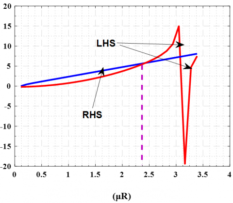
After plotting the functions LHS and RHS in Figure 4, as a function of (μR), one can observe the linearity and flatness of the RHS rather than the LHS, as the LHS is (Cot function)*. Over the range values of (μR) as shown in the figure, this property of linearity is not a common specification of the RHS function. After limiting the intersection points of the RHS with LHS, one can note that the first intersected point happened at:
$(\mu R)=2.45 R=21.7 \mathrm{~cm}, M_W=\frac{4}{3} \pi R^3=40.5 \mathrm{~kg}, M_{U 235}=1.12 \mathrm{~kg}$
*Cotangent, or cot, is a trigonometric function that represents the ratio of the adjacent side to the opposite side in a right triangle. A cot is defined as the reciprocal of the tangent function
From the figure above, one can conclude that there is little difference between the present results and the reference by Lamarsh [15]. This deviation is due to some calculation of cross sections and due to the reference using just one digit after the separator, but in the present case, having four digits after the separator, gives more accurate and real results, or the software of the previous study was different from MATLAB. It is recommended to recall several extra digits and round off the numbers only at the end of the computation.
Figure 4. The left-hand side (LHS) and right-hand side (RHS) of the two–group critical equation
R=21.7 cm, Moderator Water mass=40.5.6 kg, the fuel U235 mass=1.12 kg.
In the present case study, one can observe that the ratio of the moderator water mass to fuel U235 mass is approximately equal to 36.16, which is the same ratio for foreign reference [15], where it is equal to 36.173.
After finding the constants of the flux distribution functions, for the core and reflector, as in Eqs. (35), (36), (37), and (38), after some simplifications, it is stated that the flux distribution function is:
$\begin{gathered}\emptyset_{1 \mathrm{C}}=\mathrm{A}\left(\frac{\sin 0.113 \mathrm{r}}{\mathrm{r}}-4.67 \times 10^{-8} \frac{\sinh 0.651 \mathrm{r}}{\mathrm{r}}\right) \\ \emptyset_{2 \mathrm{C}}=0.676 \mathrm{~A}\left(\frac{\sin 0.113 \mathrm{r}}{\mathrm{r}}+3.644 .67 \times 10^{-7} \frac{\sinh 0.651 \mathrm{r}}{\mathrm{r}}\right) \\ \emptyset_{1 \mathrm{r}}=39.6 \mathrm{~A} \frac{\mathrm{e}^{-0.192 \mathrm{r}}}{\mathrm{r}}, \emptyset_{2 \mathrm{r}}=120 \mathrm{~A} \frac{\mathrm{e}^{-0.192 \mathrm{r}}}{\mathrm{r}}-21.0 \frac{\mathrm{e}^{-0.351 \mathrm{r}}}{\mathrm{r}}\end{gathered}$
From Figure 5, it is noticed that the normalization of the fluxes is to $\emptyset_{2 C}=1$, also, the largeness of the fast flux in comparison to the thermal flux, over the whole core, is gathered from the figure. The fast flux is larger than the thermal flux because the evidence points to the fact that the reactor is a thermal reactor and the core material of this reactor is extra active in absorbing thermal neutrons than in moderating neutrons out of the fast group. From the above equations, it is clear that the second term in the expression for core fluxes is small according to the first term, so the flux can be approximately written as $\emptyset_{1 \mathrm{C}} \approx \mathrm{AX}$ and $\emptyset_{2 \mathrm{C}} \approx \mathrm{AXS}_1$. Therefore the ratio of fast flux to slow flux will be:
$\begin{gathered}\frac{\emptyset_{1 C}}{\emptyset_{2 C}} \approx \frac{1}{\mathrm{~S}_1} \approx \frac{\sum_{2 \mathrm{C}}}{\sum_{1 \mathrm{C}}} \\ \frac{\emptyset_{1 \mathrm{C}}}{\emptyset_{2 \mathrm{C}}}=\frac{0.06}{0.04}=1.5 \approx \frac{1}{\mathrm{~S}_1}=1.47 \approx \frac{1}{0.676} \approx \frac{\sum_{2 \mathrm{C}}}{\sum_{1 \mathrm{C}}}=\frac{0.060}{.0419}=1.43\end{gathered}$
Figure 5. The flux of two groups for a water-moderated, water-reflected, U235 spherical reactor
The neutrons go into a diffusion process as soon as they are released.
The deep thermal core flux and the peak in the thermal reflector flux result from the thermalization of neutrons in the reflector; as indicated by the slope of the curve. At the core-reflector interface, there is a net flow of thermal neutrons from the reflector into the core.
The above phenomenon of the small peak in the fast flux within the reflector region is the most outstanding result of the group diffusion equation. This peak of thermal flux is produced by slowing down the fast neutrons, which had escaped from the core of the reflector. Some neutrons that slow down are collected in the reflector region until they are transported again to the core zone after escaping from the outer surface of the reflector or are captured.
In the real world, the theory of the occurrence of a preliminary concentration of delayed neutrons can be adjusted to the situation in which the reactor is turned off and then turned on again.
Furthermore, for future research, for constant sources of emitting neutrons with time directed to obtain a constant power level inside a nuclear reactor.
The two-group diffusion calculation is more accurate and realistic than the group diffusion equation because one group assumes that all neutrons are thermal energy and this is not true. The criticality for one group is:
$\mathrm{LHS}=\mathrm{BR} \cot \mathrm{BR}=-\frac{\mathrm{Dr}}{\mathrm{Dc}}\left(\frac{\mathrm{R}}{\mathrm{L}_{\mathrm{r}}}+1\right)=\mathrm{RHS}$,
where, B2 in cm-2 the buckling depends upon the core shape, and $L_r$ is the reflector thermal diffusion length in cm.
For our case study, the fuel density of U235 in the core is very small compared to the water moderator density. For this reason, the calculation of the group diffusion equation is more precise and logical for estimating the flux distribution, critical dimensions, and critical mass of the fuel and water.
For further application of the two-group diffusion equation, calculate the multiplication factor of a reactor configuration by adjusting the fuel concentration to meet the criticality condition. A hypothetical way of applying criticality is by reducing the concentration of the nuclear fuel and keeping the absorption cross-section constant.
I would like to express my sincere appreciation to my family, who contributed to my life. Special thanks to my supportive family. Your contributions made this project possible. Forever grateful to my family.
[1] Ajirotutu, A.D. (2020). Applications of MATLAB PDE toolbox for neutron diffusion simulation. Doctoral Dissertation, Texas A&M University-Kingsville.
[2] https://www.ans.org/news/article-5254/wna-issues-its-new-world-nuclear-performance-report/.
[3] Irkimbekov, R., Vurim, A., Vityuk, G., Zhanbolatov, O., Kozhabayev, Z., Surayev, A. (2023). Modeling of dynamic operation modes of IVG. 1M reactor. Energies, 16(2): 932. https://doi.org/10.3390/en16020932
[4] Farman, N.F., Mahdi, S.A., Redha, Z.A.A. (2017). Mathematical analysis of the transient dynamic of surge-in or/and surge-out of the pressurizer of PWR. International Journal of Simulation-Systems, Science & Technology, 18(4): 5.1-5.20. https://doi.org/10.5013/IJSSST.a.18.04.05
[5] Mahdi, S.A., Farman, N.F., Redha, Z.A.A. (2018). Genetic algorithms to estimate the pressure deviations in dynamic transients of the pressurizer response in PWRs. International Journal of Simulation-Systems, Science & Technology, 19(1): 3.1-3.12. https://doi.org/10.5013/IJSSST.a.19.01.03
[6] Farman, N.F., Mahdi, S.A., Redha, Z.A.A. (2018). A review of advances in pressurizer response research for pressurized water reactor systems. International Journal of Simulation-Systems, Science & Technology, 19(2): 3.1-3.11. https://doi.org/10.5013/IJSSST.a.19.02.03
[7] Knife, R.A. (2014). Nuclear Engineering: Theory and Technology of Commercial Nuclear Power. 2nd Ed.
[8] Smith, K.S. (1979). An analytic nodal method for solving the two-group, multidimensional, static and transient neutron diffusion equations. Doctoral Dissertation, Massachusetts Institute of Technology.
[9] Melo, F.D.S., Cabral, R.G., Conti Filho, P. (2009). Analytical versus discretized solutions of four-group diffusion equations to thermal reactors. 2009 International Nuclear Atlantic Conference - INAC 2009 Rio De Janeiro, Brazil, September 27 to October 2, 2009.
[10] Hosseini S.A. (2016). 3D neutron diffusion computational code based on GFEM with unstructured tetrahedron elements: A comparative study for linear and quadratic approximations. Energy, 92: 119-132. https://doi.org/10.1016/j.pnucene.2016.07.006
[11] Shqair, M., El-Ajou, A., Nairat, M. (2019). Analytical solution for multi-energy groups of neutron diffusion equations by a residual power series method. Mathematics, 7(7): 633. https://doi.org/10.3390/math7070633
[12] Shqair, M., El-Zahar, E.R. (2020). Analytical solution of neutron diffusion equation in reflected reactors using modified differential transform method. In: Zeidan, D., Padhi, S., Burqan, A., Ueberholz, P. (eds) Computational Mathematics and Applications. Forum for Interdisciplinary Mathematics. Springer, Singapore. https://doi.org/10.1007/978-981-15-8498-5_6
[13] Jevremovic, T. (2009). Nuclear Principles in Engineering (Vol. 2). US: Springer. https://doi.org/10.1007/978-0-387-85608-7
[14] Lamarsh, J.R., Baratta, A.J. (2001). Introduction to Nuclear Engineering (Vol. 3, p. 783). Upper Saddle River, NJ: Prentice-Hall, Inc.
[15] Lamarsh, J.R. (1972). Nuclear Reactor Theory. 2nd Ed. Addison-Wesley Company.
[16] Holmes, D.K., Meghreblian, R.V. (1955). Notes on Reactor Analysis. Part II. Theory (No. CF-54-7-88 (Pt. II)). Oak Ridge National Lab., Tenn. (US).