Samson A. Adeleye![]() | Taiwo O. Oni*
| Taiwo O. Oni*![]() | Iyiola O. Oluwaleye
| Iyiola O. Oluwaleye![]()
© 2023 IIETA. This article is published by IIETA and is licensed under the CC BY 4.0 license (http://creativecommons.org/licenses/by/4.0/).
OPEN ACCESS
Heat transfer and fluid flow in cavities is often a result of convection. The study of convection in enclosures, such as rectangular cavities, under different parameters, holds significance in understanding the thermal-hydraulic characteristics, like temperature and air velocity distribution, in systems where heat transfer and fluid flow are involved. This research focuses on the numerical investigation of temperature and air velocity distribution in a rectangular cavity. COMSOL Multiphysics software was utilized to create a model of the cavity, subjecting it to regulated temperatures of 323.0 K, 333.0 K, and 343.0 K at operating times of 0, 300, 900, and 1,500 seconds. The cavity's bottom wall was heated by a heater, and the inner sides of the right and left walls were insulated using fiberglass. The findings from the research indicate that at an operating time of 900 seconds, the maximum air velocities recorded were 0.06, 0.06, 0.03, and 0.10 m/s at the left wall, right wall, bottom, and top of the cavity respectively. Beyond 900 seconds of operation, the air velocities remained constant. Furthermore, at 900 seconds of operation, the maximum isotherms at the regulated temperatures of 323.0 K, 333.0 K, and 343.0 K were approximately equal to their respective temperatures, but they precisely equaled the regulated temperatures at an operating time of 1,500 seconds. The results of this research can be applied to various areas that involve heat and fluid flow, including heat exchangers, building design for energy efficiency, solar systems, nuclear reactor operations, microelectronic component cooling, energy storage, heating devices, and refrigeration systems.
cavity, simulation, temperature, time, velocity, wall
Heat transfer and fluid flow in cavities are predominantly governed by convective processes [1]. Convective heat transfer ensues when a fluid, heated and thus less dense, ascends, leading to the displacement of the cooler surrounding fluid. As the cooler fluid is subsequently warmed, it too becomes less dense and rises, paving the way for the cooler fluid to replace it, thereby engendering a convective current [1, 2].
The centrality of convective phenomena in numerous engineering applications has spurred considerable research interest. Significant strides have been made in recent years in elucidating the underlying physical processes involved in convection, driven in part by the advent of robust numerical methods, which have facilitated the analysis of convective phenomena in cavities [3].
Applications encompassing convective processes are ubiquitous, ranging from energy-efficient building design, solar systems, and nuclear reactor operations to energy storage, multi-pane window heat transfer, heating devices, and refrigeration systems [1, 4].
Numerous studies have sought to probe the influence of various input variables on system outputs across diverse enclosure geometries, employing both theoretical and experimental approaches. For instance, numerical investigations have been conducted on convection within rectangular enclosures, both with and without heat generation, revealing distinct isotherm and flow patterns [5]. Similarly, convection between two horizontal concentric elliptic cylinders has been numerically analyzed, shedding light on the heat transfer characteristics and flow patterns under various conditions [6].
Research has also delved into convective phenomena within open cavities, where a uniform heat flux was applied to the slotted wall facing the opening [7]. Employing the finite difference-control volume method to solve the conservation equations, it was found that the Nusselt number and volume flow rate increased with increasing Rayleigh number, but decreased as the number of slots increased.
Further numerical investigations have been carried out on rectangular enclosures heated from below and cooled from above, considering various ratios of the shorter to the longer length of the enclosures (r) and Rayleigh number values based on enclosure height [8]. The findings suggested that these ratios and Rayleigh numbers could be harnessed to optimize heat transfer within the enclosure.
In a similar vein, a rectangular enclosure heated from below with symmetrically cooled sides has been investigated. Notably, due to the symmetry of the boundary conditions in the vertical direction, both the flow and temperature fields were found to be symmetrical along the enclosure's midpoint [9].
Investigations into convective air movement in rectangular enclosures under varying conditions have been undertaken, including scenarios where two or more adjacently situated walls were differentially heated, or where disparate portions of the same wall were maintained at non-uniform temperatures [10]. These investigations considered different values of the enclosure's height-to-width ratio, the Rayleigh number, and the heated fractions of the sidewalls.
Several findings emerged from these studies. For instance, increases in both the Hartmann number and internal Rayleigh number were found to decrease the convective heat transmission rate [11]. Furthermore, a stronger magnetic field was observed to decrease the average Nusselt number [11]. Additional research has employed a constrained interpolated profile method to simulate natural convection heat transfer and fluid flow in a square enclosure with differentially heated sidewalls [12]. Here, the velocity and temperature profiles for varying Rayleigh numbers were compared with lattice-Boltzmann formulations.
Steady-state conjugate convection in a rectangular enclosure has also been numerically analyzed [13]. In these studies, discrete heat sources were applied to one of the vertical walls, with air and dielectric fluorocarbon liquids serving as working fluids. The results revealed that increases in the Rayleigh number corresponded to increases in both the dimensionless heat flux and the Nusselt number for both fluids. Moreover, the dimensionless temperature at the interface between the enclosure walls and the fluids was found to increase as the Rayleigh number decreased.
Other investigations have focused on convection within trapezoidal enclosures filled with nanotubes [14]. After simulations were run for a variety of ratios of different lengths and heights of the enclosure, it was concluded that at a low Rayleigh number, the average Nusselt number decreased when the inclination angle was increased, independent of solid volume fractions. Furthermore, the Rayleigh number was observed to increase as buoyancy forces became dominant.
Finally, research has been conducted on convective flows and heat transfer induced within a vertical row of heated horizontal cylinders [15]. Flow visualizations were plotted to understand the results. Two different configurations were numerically investigated [16]. In one configuration, a uniform heat flux was applied to a wet wall, while in the second configuration, the same heat flux preheated the liquid at the inlet. The latter configuration was found to increase the evaporation rate.
Comparative analyses of heat transfer performances for a spider-netted microchannel and a straight microchannel were conducted for heat flux values ranging from 10 to 100 W/cm2 [17]. Findings from these analyses elucidated that, for identical heat flux values, the spider-netted microchannel yielded a higher heat transfer coefficient and exhibited a lower superheat temperature than the straight microchannel.
Investigations have been carried out concerning the correlation of heat transfer coefficients during poly-phase transformations within and outside a tube [18]. It was demonstrated that an increase in feed flow speed and ethanol content within the tube led to an increase in the heat transfer coefficient. Conversely, an increase in the temperature difference between the tube's interior and exterior resulted in a decrease in the heat transfer coefficient.
A multi-fluid model for resolving subcooled flow boiling was also proposed [19]. It was reported that a two-phase rough wall function, as compared to a classical single-phase wall function, yielded a more reliable estimate of the radial velocity profile.
Further research explored the impact of dried ice particles formed into hard chunks on heat transfer within a fluidized bed [20]. Findings indicated enhanced ice particle mixing when fluid velocity was increased.
Studies have also examined shallow flow past a channel lateral cavity [21]. Utilizing a non-intrusive method to measure the water surface in the cavity region of the channel, velocity fields were presented.
Convection heat transfer within a differentially heated cavity was considered [22]. The Lattice Boltzmann method was employed to ascertain the effects of heat source-sink pair sizes, numbers, and arrangements on flow and thermal fields. Results indicated that the arrangement of these heat source-sink pairs significantly influenced the flow and thermal fields within the cavity.
Despite the extensive research on heat transfer characteristics in various cavities as detailed above, a dearth of literature exists on the velocity and temperature distribution within a cavity. Therefore, this study aims to numerically investigate the effects of regulated temperatures on air velocity and temperature distributions within a rectangular cavity, considering regulated temperatures of 323.0K, 333.0K, and 343.0K. This work is poised to contribute significantly to research in heat and fluid flow. It was found that air velocity within the cavity increased with operating time, although this increase plateaued beyond 900 seconds. Concurrently, the temperature within the cavity exhibited an increase with both operating time and regulated temperature.
2.1 Geometry of the rectangular cavity
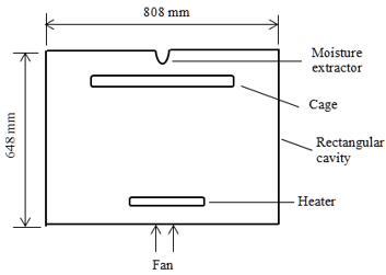
The rectangular cavity is shown in Figure 1. Its dimensions are 808 mm×648 mm, and it is made of gauge 18-sheet galvanized steel. The cavity contains a cage of dimensions 720 mm×350 mm. A fan is attached to the bottom of the cavity to draw air into it. A moisture extractor is fixed on the top of the cavity to allow for the escape of air from the cavity. A heater, which is made of copper, is installed inside the cavity to supply heat to it. The left and right sides of the inner wall of the cavity are made of a fiberglass insulator to reduce heat loss through the walls.
Figure 1. Geometry of the rectangular cavity
2.2 Governing equations
The governing equations for the flow of air in the rectangular cavity are given as follows:
Continuity equation:
$\frac{\partial u}{\partial x}\,\,+\,\,\frac{\partial v}{\partial y}\,\,=\,\,0$ (1)
Conservation of momentum in x direction:
$u \cdot \frac{\partial u}{\partial x}+v \cdot \frac{\partial u}{\partial y}\,\,=\,\,-\frac{1}{\rho} \cdot \frac{\partial p}{\partial x}\,\,+\,\,\frac{\mu}{\rho}\,\,\left(\frac{\partial^2 u}{\partial x^2}\,\,+\,\,\frac{\partial^2 u}{\partial y^2}\right)$ (2)
Conservation of momentum in y direction:
$u \cdot \frac{\partial v}{\partial x}\,\,+\,\,v \cdot \frac{\partial v}{\partial y}\,\,=\,\,-\,\,\frac{1}{\rho} \cdot \frac{\partial p}{\partial y}\,\,+\,\,\frac{\mu}{\rho}\left(\frac{\partial^2 v}{\partial x^2}\,\,+\,\,\frac{\partial^2 v}{\partial y^2}\right)$ (3)
Energy equation:
$\frac{\partial \theta}{\partial t}\,\,+\,\,u \cdot \frac{\partial \theta}{\partial x}\,\,+\,\,v \cdot \frac{\partial \theta}{\partial y}\,\,=\,\,\frac{k}{\rho C_p}\left(\frac{\partial^2 \theta}{\partial x^2}\,\,+\,\,\frac{\partial^2 \theta}{\partial y^2}\right)$ (4)
where, ρ is the density (kg⁄m3), θ is the temperature (K), p is the pressure (Pa), µ is the dynamic viscosity (kg⁄ms), k is thermal conductivity (W⁄(m.K)), u is the horizontal components of the velocity of flow (m/s), and v is vertical components of the velocity of flow (m/s). In this study, it is assumed that the fluid flow is steady and not compressible, and the fluid is Newtonian.
2.3 Boundary conditions
The boundary conditions are air inlet temperature, θo=298K, different regulated temperatures, θ=323.0K, 333.0K, 343.0K, and heat source, s=9,000W. The values of other parameters used as boundary conditions, as obtained from Bergman et al. [23], are the density of air at the inlet, ρ=1 kg⁄m3; the specific heat capacity of fiberglass at constant pressure, CP,f=1 J/kgK; the specific heat capacity of aluminum at constant pressure, CP,a=893 J/kgK; the specific heat capacity of copper at constant pressure, CP,c= 385J/kgK; the specific heat capacity of steel at constant pressure, CP,s=475 J/kgK.
2.4 Numerical method
Simulations were carried out by means of COMSOL Multiphysics software. The finite element in the software was used to solve the partial differential equations by subdividing the problem into smaller and simpler parts (that is, finite elements) through a process known as discretization. The finite elements form an interconnected network of concentrated nodes and use the predefined equations of the solver to calculate the values at every node.
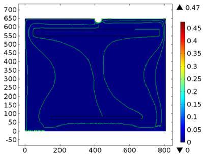
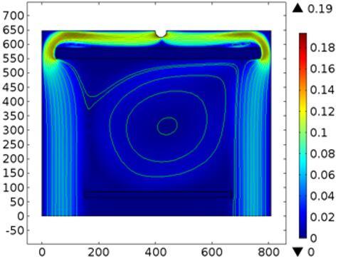
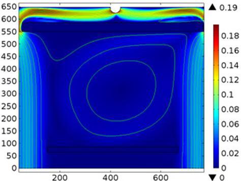
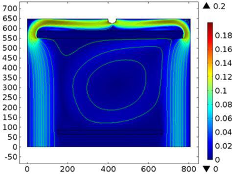
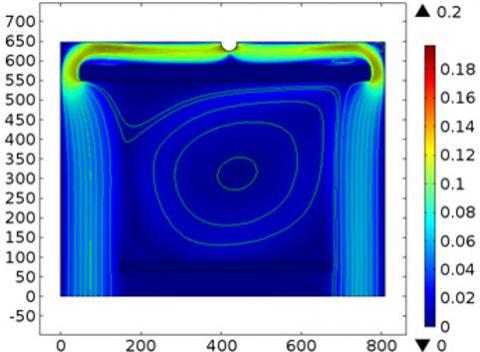
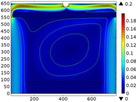
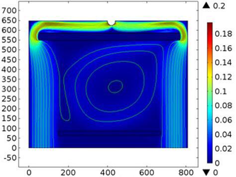
The contour of distribution of air velocity (m/s) in the cavity for operating times of 0, 300, 900, and 1,500 seconds, and at a regulated temperature of 323.0 K, 333.0 K, and 343.0 K are shown in Figure 2-Figure 5.
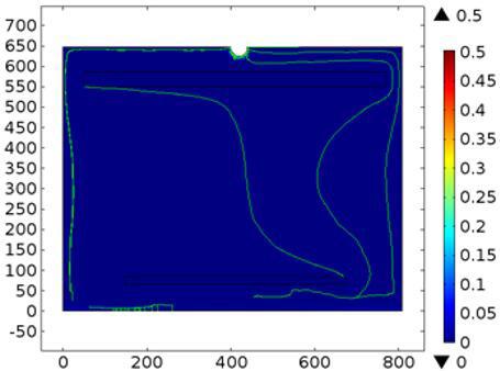
At a time of 0 seconds for the regulated temperature of 323.0 K, 333.0 K, and 343.0 K (Figure 2), the velocity in the cavity is 0.05m/s. When the time was increased to 300 seconds, as shown in Figure 3, the velocity at the left and right walls of the cavity is 0.06 m/s for the regulated temperature of 323.0 K (Figure 3(a)), 333.0 K (Figure 3(b)), and 343.0 K (Figure 3(c)), compared with the case of the time of 0 seconds (Figure 2). The increase in the velocity is as a result of velocity buildup with advance of time. The maximum value of the velocity at the top of the cavity is 0.10 m/s, but it is 0.02 m/s at its bottom for the regulated temperature of 323.0 K (Figure 3(a)). For the regulated temperature of 333.0 K (Figure 3(b)), the cavity has a maximum velocity of 0.10 m/s at its top and 0.02 m/s at its bottom. The maximum value of the velocity at the top of the cavity is 0.10 m/s, but it is 0.02 m/s at its bottom for the regulated temperature of 343.0 K (Figure 3(c)). It is therefore revealed that there is an increase in the velocity at the bottom and top of the cavity, compared with that of the case when the time was 0 second.
(a)
(b)
(c)
Figure 2. Distribution of velocity (m/s) at time = 0 second for regulated temperature (a) 323.0K (b) 333.0K, and (c) 343.0K
(a)
(b)
(c)
Figure 3. Distribution of velocity (m/s) at time = 300 seconds for regulated temperature (a) 323.0 K (b) 333.0 K, and (c) 343.0 K
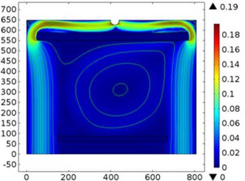
At the time of 900 seconds (as shown in Figure 4), the velocity at the left and right walls of the cavity is 0.06 m/s for the regulated temperature of 323.0 K (Figure 4(a)), 333.0 K (Figure 4(b)), and 343.0 K (Figure 4(c)), compared with the case of the time of 300 seconds (Figure 3). The maximum value of the velocity at the top of the cavity is 0.13 m/s, but it is 0.03 m/s at its bottom for the regulated temperature of 323.0K (Figure 4(a)). For the regulated temperature of 333.0K (Figure 4(b)), the cavity has a maximum velocity of 0.13 m/s at its top and 0.03 m/s at its bottom. The maximum value of the velocity at the top of the cavity is 0.15 m/s, but it is 0.03 m/s at its bottom for the regulated temperature of 343.0 K (Figure 4(c)). This means that there is an increase in the velocity at the bottom and top of the cavity, compared with that of the case when the time was 300 seconds. The rise in the velocity as the regulated temperature increases is a consequence of the decrease in the density of the air as the temperature increases.
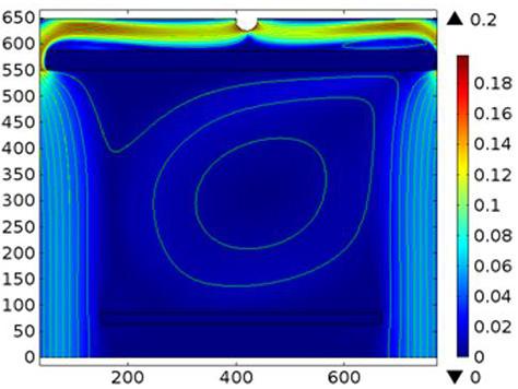
Figure 5 shows that when the time was increased to 1,500 seconds, the velocity at the left and right walls of the cavity is 0.06 m/s for the regulated temperature of 323.0 K (Figure 5(a)), 333.0 K (Figure 5(b)), and 343.0 K (Figure 5(c)). The velocity in the cavity has a maximum value of 0.10 m/s at its top, whereas it is 0.03 m/s at its bottom for the regulated temperature of 323.0K (Figure 5(a)). It has a maximum value of 0.13 m/s at its top, and a maximum value of 0.03 m/s at its bottom for the regulated temperature of 333.0 K (Figure 5(b)). The maximum value of the velocity at the top of the cavity is 0.13 m/s, but it is 0.03 m/s at its bottom for the regulated temperature of 343.0 K (Figure 5(c)). Thus, it can be seen that the values obtained for the time of 1,500 seconds are the same as those for the time of 900 seconds.
(a)
(b)
(c)
Figure 4. Distribution of velocity (m/s) at time = 900 seconds for regulated temperature (a) 323.0 K (b) 333.0 K, and (c) 343.0 K
3.2 Temperature distribution of air
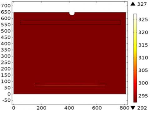
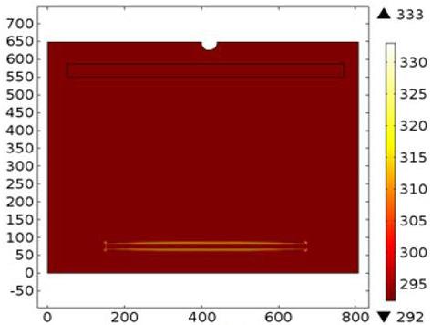
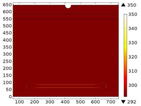
The temperature distribution of air in the rectangular cavity for the time of 0, 300, 900, and 1,500 seconds at a regulated temperature of 323.0 K, 333.0 K, and 343.0 K are presented in this section. At the time of 0 second (Figure 6), the temperature in the cavity is constant, being 303.0 K, 307.0 K, and 312.0 K for the regulated temperature of 323.0 K, 333.0 K, and 343.0 K respectively.
(a)
(b)
(c)
Figure 5. Distribution of velocity (m/s) at time = 1,500 seconds for regulated temperature (a) 323.0 K (b) 333.0 K, and (c) 343.0 K
(a)
(b)
(c)
Figure 6. Temperature (K) at time=0 second and at a regulated temperature (a) 323.0 K (b) 333.0 K, and (c) 343.0 K
Figure 7 indicates that at the time of 300 seconds, the maximum and minimum temperatures are 315.0 K and 305.0 K, respectively, for the regulated temperature of 323.0 K (Figure 7(a)); 320.0 K and 310.0 K, respectively, for the regulated temperature of 333.0 K (Figure 7(b)); and 325.0 K and 315.0 K, respectively, for the regulated temperature of 343.0 K (Figure 7(c)).
(a)
(b)
(c)
Figure 7. Temperature (K) at time = 300 seconds and at a regulated temperature (a) 323.0 K (b) 333.0 K, and (c) 343.0 K
(a)
(b)
(c)
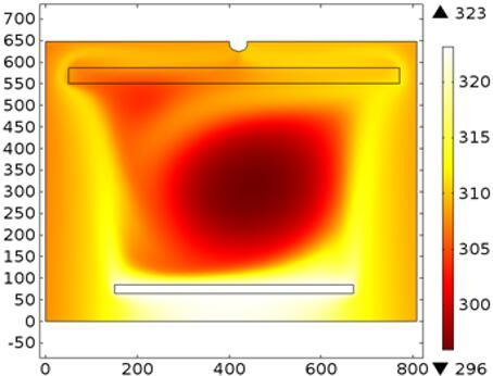
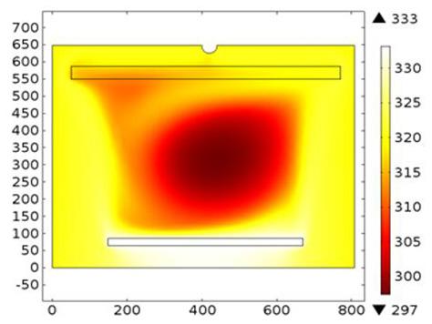
Figure 8. Temperature (K) at time=900 seconds and at a regulated temperature (a) 323.0 K (b) 333.0 K, and (c) 343.0 K
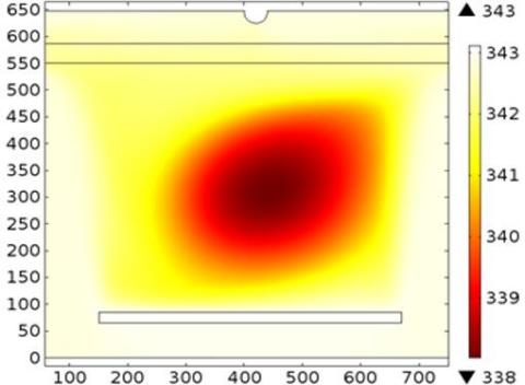
In addition, it can be seen in Figure 8 that at the time of 900 seconds, the maximum and minimum temperatures are 320.0 K and 314.0 K, respectively, for the regulated temperature of 323.0 K (Figure 8(a)); 330.0 K and 324.0 K, respectively, for the regulated temperature of 333.0 K (Figure 8(b)); and 338.0 K and 330.0 K, respectively, for the regulated temperature of 343.0K (Figure 8(c)). The increase in the temperature in the cavity is a result of the growth of heat in the cavity due to the increase in the operating time and regulated temperature. At the time of 1,500 seconds (Figure 9), the maximum and minimum temperatures are 322.0 K and 321.0 K, respectively, for the regulated temperature of 323.0 K (Figure 9(a)); 332.0K and 331.0 K, respectively, for the regulated temperature of 333.0 K (Figure 9(b)); and 342.0 K and 340.0 K, respectively, for the regulated temperature of 343.0 K (Figure 9(c)).
(a)
(b)
(c)
Figure 9. Temperature (K) at time = 1,500 seconds and at a regulated temperature (a) 323.0 K (b) 333.0 K, and (c) 343.0 K
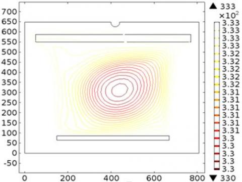
3.3 Isotherms
Isotherms represent the lines of constant temperature in the cavity. Isotherms are one of the means that can be used to represent flow and heat transfer characteristics in cavities. The contours of the isotherms for the regulated temperature of 323.0 K, 333.0 K, and 343.0 K are shown in Figure 10-Figure 13.
(a)
(b)
(c)
Figure 10. Isotherm at time = 0 second and at a regulated temperature (a) 323.0 K (b) 333.0 K, and (c) 343.0 K
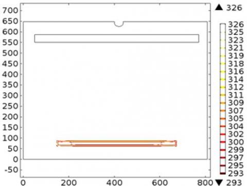
At the time of 0 second (Figure 10), the isotherm in the cavity for the regulated temperature of 323.0K Figure 10(a)), 333.0K (Figure 10(b)), and 343.0 K (Figure 10(c)) is 298.0 K. It is shown in Figure 11 that at the time of 300 seconds, the maximum and minimum isotherms are 320.0 K and 310.0 K, respectively, for the regulated temperature of 323.0 K (Figure 11(a)); 330.0 K and 314.0 K, respectively, for the regulated temperature of 333.0 K (Figure 11(b)); and 340.0 K and 319.0 K, respectively, for the regulated temperature of 343.0 K (Figure 11(c)).
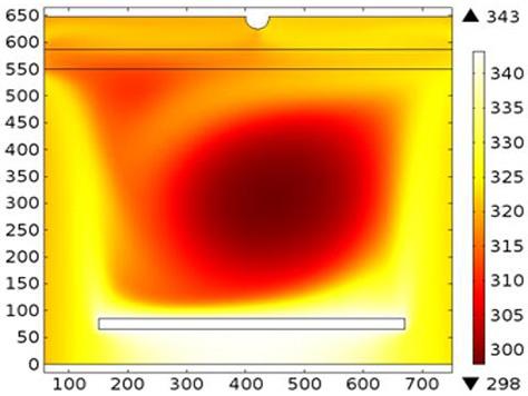
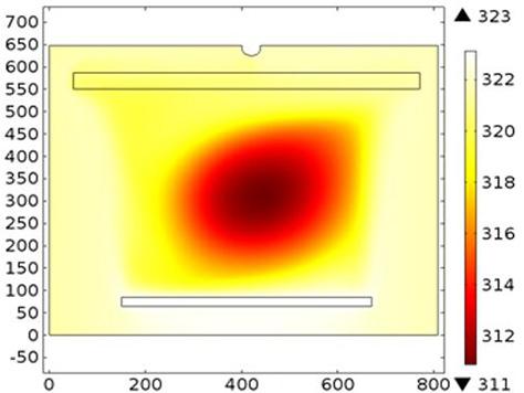
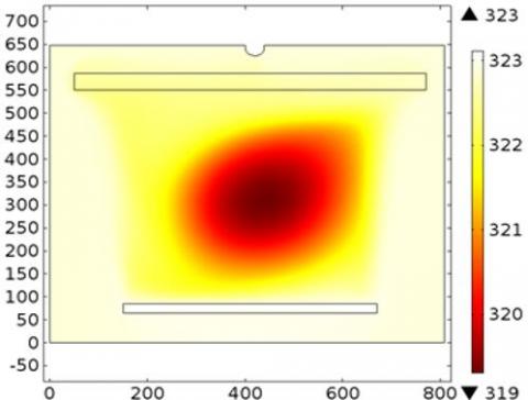
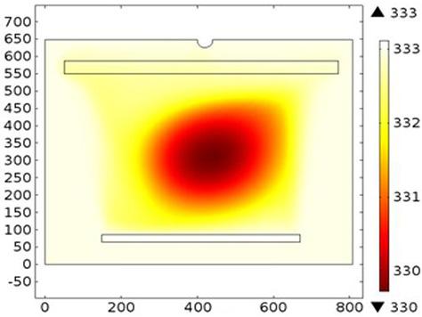
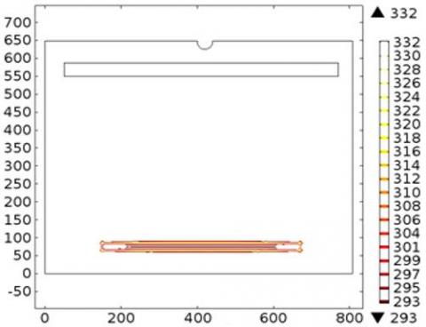
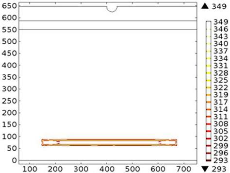
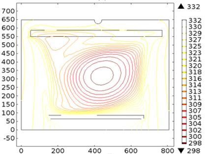
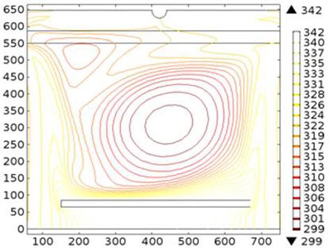
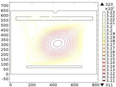
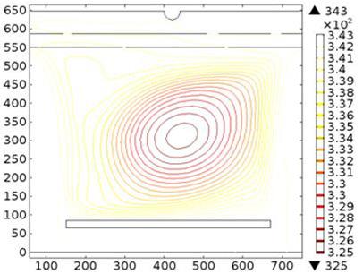
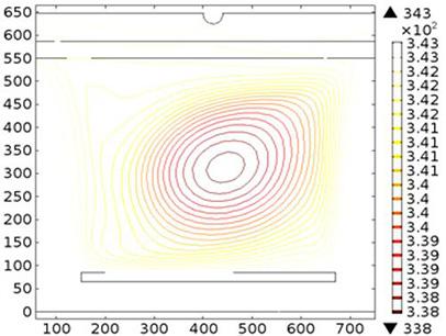
At the time of 900 seconds (represented by Figure 12), the maximum and minimum isotherms are 322.0 K and 317.0 K, respectively, for the regulated temperature of 323.0K (Figure 12(a)); 332.0 K and 326.0 K, respectively, for the regulated temperature of 333.0 K (Figure 12(b)); and 342.0 K and 333.0 K, respectively, for the regulated temperature of 343.0 K (Figure 12(c)). It is displayed in Figure 13 that at the time of 1,500 seconds, the maximum and minimum isotherms are 323.0 K and 321.0 K, respectively, for the regulated temperature of 323.0 K (Figure 13(a)); 333.0 K and 332.0 K, respectively, for the regulated temperature of 333.0 K (Figure 13(b)); and 343.0 K and 341.0 K, respectively, for the regulated temperature of 343.0 K (Figure 13(c)).
(a)
(b)
(c)
Figure 11. Isotherm at time = 300 seconds and at a regulated temperature (a) 323.0 K (b) 333.0 K, and (c) 343.0 K
It can be observed that at the time of 900 seconds, the maximum isotherms are 322.0 K, 332.0 K, and 342.0 K for the regulated temperature of 323.0 K, 333.0K, and 343.0 K, respectively. This means that the maximum isotherms are approximately equal to the regulated temperature at the time of 900 seconds. Interestingly, at the time of 1,500 seconds, the maximum isotherm at the regulated temperature of 323.0 K, 333.0 K, and 343.0 K is exactly equal to 323.0 K, 333.0 K, and 343.0 K, respectively.
(a)
(b)
(c)
Figure 12. Isotherm at time = 900 seconds and at a regulated temperature (a) 323.0 K (b) 333.0 K, and (c) 343.0 K
3.4 Validation of the simulation results with experimental results
It is important to ensure that the results of the simulation are reliable. Therefore, the results of the simulation were validated with the results obtained from the experiments that were performed on them, as presented below.
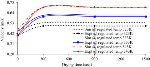
Velocity distribution. The validation of the simulated results of the velocity with their experimental results at the different regulated drying temperatures is shown in Figure 14. The standard deviations of the velocity between the simulated results and their experimental results for the regulated drying temperature of 323 K at the operating time of 0, 300, 900, and 1,500 seconds are 0.033, 0.024, 0.025, and 0.025 m/s, respectively. They are 0.033, 0.010, 0.012, and 0.012 m/s at the operating time of 0, 300, 900, and 1,500 seconds, respectively, for the regulated drying temperature of 333 K.
When the regulated drying temperature was 343 K, the standard deviations are 0.046, 0.001, 0.001, and 0.001 m/s at the time of 0, 300, 900, and 1,500 seconds, respectively. The values of the standard deviations indicate that the simulated results and the experimental results are in good harmony with one another and confirm that the simulated results are reliable.
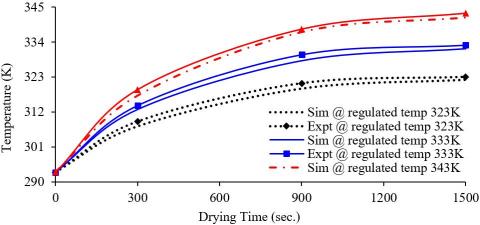
Temperature distribution. The validation of the simulated results of the temperature with their experimental results at the different regulated drying temperatures is shown in Figure 15. When the regulated drying temperature was 323 K, the standard deviations are 0.11, 1.09, 1.20, and 0.65K at the time of 0, 300, 900, and 1,500 seconds, respectively. The standard deviations are 0.11, 0.89, 1.38, and 0.84 K at the operating time of 0, 300, 900, and 1,500 seconds, respectively, for the regulated drying temperature of 333 K. The simulated and experimental results for the regulated drying temperature of 343 K at the operating time of 0, 300, 900, and 1,500 seconds have standard deviations of 0.11, 1.34, 0.67, and 0.96 K, respectively. As with the case of the velocity, the simulated and the experimental results are in good agreement with one another.
(a)
(b)
(c)
Figure 13. Isotherm (K) at time = 1,500 seconds and at a regulated temperature (a) 323.0 K (b) 333.0 K, and (c) 343.0 K
Figure 14. Validation of the simulated results of the velocity with the experimental results
Figure 15. Validation of the simulated results of the temperature with the experimental results
Numerical simulation was carried out to study the effects of regulated temperatures on the distribution of air velocity and temperature in a rectangular cavity. The regulated temperatures considered are 323.0K, 333.0K, and 343.0K, each for operating times of 0, 300, 900, and 1,500 seconds.
The air velocity in the cavity increases as operating the time increases. The rise in the velocity as the regulated temperature increases is a consequence of the decrease in the density of the air as the temperature increases. From the time of 900 seconds upward, the velocity of air does not change.
The temperature distribution shows that the temperature in the cavity rises as the operating time rises. Also, it rises as the regulated temperature rises. The increase in the temperature in the cavity is a result of the growth of heat in the cavity due to the increase in the operating time and regulated temperature.
The maximum isotherms are approximately equal to the regulated temperatures of 323.0K, 333.0K, and 343.0K at the time of 900 seconds, but are exactly equal to the regulated temperatures at the time of 1,500 seconds.
The validation of the simulated results with experimental results reveals a good harmony among them, and, therefore, the reliability of the simulations.
The research in this paper can be meaningfully applied in the design of and the monitoring of processes in heat transfer and fluid flow systems.
|
Cp |
specific heat, J. kg-1. K-1 |
|
k |
thermal conductivity, W. m-1. K-1 |
|
s |
heat source, W (W) |
|
u |
horizontal component of velocity of flow, m-1. s-1 |
|
v |
vertical component of velocity of flow, m-1. s-1 |
|
ρ |
density, kg-1. m-3 |
|
θ |
Temperature, K |
[1] Holman, J.P. (2010). Heat Transfer. McGraw Hill Companies, Inc., New York.
[2] Azwadi, C.S., Tanahashi, T. (2006). Simplified thermal lattice Boltzmann in incompressible limit. International Journal of Modern Physics, 20(17): 2437-2449. https://doi.org/10.1142/S0217979206034789
[3] Abu-Nada, E., Oztop, H.F. (2009). Effects of inclination angle on natural convection in enclosures filled with Cu-water nanofluid. International Journal of Heat and Fluid Flow, 30(4): 669-678. https://doi.org/10.1016/j.ijheatfluidflow.2009.02.001
[4] Ahmadi, M. (2014). Fluid flow and heat transfer characteristics of natural convection in square 3-D enclosure due to discrete sources. World Applied Sciences Journal, 29(10): 1291-1300. https://doi.org/10.5829/idosi.wasj.2014.29.10.1578
[5] Rahman, M., Sharif, M.A.R. (2003). Numerical study of laminar natural convection in inclined rectangular enclosures of various aspect ratios. Numerical Heat Transfer - Part A: Applications, 44(4): 355-373. https://doi.org/10.1080/713838233
[6] Zhu, Y.D., Shu, C., Qiu, J., Tani, J. (2004). Numerical simulation of natural convection between two elliptical cylinders using DQ method. International Journal of Heat and Mass Transfer, 47: 797-808. https://doi.org/10.1016/j.ijheatmasstransfer.2003.06.005
[7] Bilgen, E., Muftuoglu, A. (2008). Natural convection in an open square cavity with slots. International Communications in Heat and Mass Transfer, 35(8): 896-900. https://doi.org/10.1016/j.icheatmasstransfer.2008.05.001
[8] Moghimi, S.M., Mirgolbabaei, H., Miansari, M. (2009). Natural convection in rectangular enclosures heated from below and cooled from above. Australian Journal of Basic and Applied Sciences, 3(4): 4618-4623.
[9] Basak, T., Roy, S., Sharma, P.K., Pop, I. (2009). Analysis of mixed Convection within a square cavity with linearly heated side wall(s). International Journal of Heat and Mass Transfer, 52(9-10): 2224-2242. https://doi.org/10.1016/j.ijheatmasstransfer.2008.10.033
[10] Caronna, G., Corcione, M., Habib, E. (2009). Natural convection heat and momentum transfer in rectangular enclosures heated at the lower portion of the sidewalls and the bottom wall and cooled at the remaining upper portion of the sidewalls and the top wall. Heat Transfer Engineering, 30(14): 1166-1176. https://doi.org/10.1080/01457630902972777
[11] Obayedullah, M., Chowdhury, M.M.K., Rahman, M.M. (2013). Natural convection in a rectangular cavity having internal energy sources and electrically conducting fluid with sinusoidal temperature at the bottom wall. International Journal of Mechanical and Materials Engineering, 8(1): 73-78.
[12] Mitra, A. (2013). Numerical study of natural convection in an enclosed square cavity using Constrained Interpolated Profile (CIP) method. International Journal of Research in Engineering and Technology, 2(9): 18-25. https://doi.org/10.15623/ijret.2013.0209003
[13] Gdhaidh, F.A., Hussain, K., Qi, H.S. (2014). Numerical investigation of conjugate natural convection heat transfer from discrete heat sources in rectangular enclosure. World Congress on Engineering 2014, London, U.K., pp. 1304-1309.
[14] Esfe, M.H., Arani, A.A.A., Yan, W.M., Ehteram, H., Aghaie, A., Afrand, M. (2016). Natural Convection in trapezoidal enclosure filled with carbon nanotube-EG-water Nanofluid. International Journal of Heat and Mass Transfer, 92: 76-82. https://doi.org/10.1016/j.ijheatmasstransfer.2015.08.036
[15] Kitamura, K., Mitsuishi, A., Suzuki, T., Kimura, F. (2016). Fluid flow and heat transfer of natural convection induced around a vertical row of heated horizontal cylinders. International Journal of Heat and Mass Transfer, 92: 414-429. https://doi.org/10.1016/j.ijheatmasstransfer.2015.08.086
[16] Alla, A.N., Feddaoui, M., Meftah, H. (2018). Comparison of two configurations to improve heat and mass transfer in evaporating two-component liquid film flow. International Journal of Thermal Sciences, 126: 194-204. https://doi.org/10.1016/j.ijthermalsci.2017.12.031
[17] Tan, H., Chen, J., Wang, M., Du, P. (2018). Experimental study of flow boiling heat transfer in spider netted microchannel for chip cooling. The World Congress on Engineering 2018, London, U.K., pp. 708-711.
[18] Fang, J., Li, K., Diao, M. (2019). Establishment of the falling film evaporation model and correlation of the overall heat transfer coefficient. Royal Society Open Science, 6(5): 1-16. https://doi.org/10.1098/rsos.190135
[19] Amidu, M.A., Addad, Y., Riahi, M.K. (2020). A hybrid multiphase flow model for the prediction of both low and high void fraction nucleate boiling regimes. Applied Thermal Engineering, 178: 115625. https://doi.org/10.1016/j.applthermaleng.2020.115625
[20] Garcia-Gutierrez, L.M., Hernández-Jiménez, F., Cano-Pleite, E., Soria-Verdugo, A. (2020). Experimental evaluation of the convection heat transfer coefficient of large particles moving freely in a fluidized bed reactor. International Journal of Heat and Mass Transfer, 153: 119612. https://doi.org/10.1016/j.ijheatmasstransfer.2020.119612
[21] Navas-Montilla, A., Martinez-Aranda, S., Lozano, A., Garcia-Palacin, I., Garcia-Navarro, P. (2021). 2D experiments and numerical simulation of the oscillatory shallow flow in an open channel lateral cavity. Advances in Water Resources, 148: 103836. https://doi.org/10.1016/j.advwatres.2020.103836
[22] Dadvand, A., Saraei, S.H., Ghoreishi, S., Chamkha, A.J. (2021). Lattice Boltzmann simulation of natural convection in a square enclosure with discrete heating. Mathematics and Computers in Simulation, 179: 265-278. https://doi.org/10.1016/j.matcom.2020.07.025
[23] Bergman, T.L., Lavine, A.S., Incropera, F.P., Dewitt, D.P. (2011). Fundamentals of Heat and Mass Transfer. John Wiley & Sons Inc., USA.