Yousuf Alhendal*![]() | Sara Touzani
| Sara Touzani![]()
© 2023 IIETA. This article is published by IIETA and is licensed under the CC BY 4.0 license (http://creativecommons.org/licenses/by/4.0/).
OPEN ACCESS
This study presents an experimental and numerical investigation into the thermofluid characteristics of airflow over an inclined, heated plate, mimicking a solar panel. The inclination of the plate was systematically adjusted from 0° to 90°, and the heat flux was varied from 1000 to 4000 W/m², with Reynolds number ranging from 63,000 to 650,000. The study employed a second-order finite volume method for discretization and resolution of steady fluid dynamics problems, with simulations conducted using Ansys Fluent software. The k-ε RNG turbulence model was utilized for these simulations. The numerical results, validated against experimental data, were extrapolated to assess the behaviour at a wide range of attack angles and flow rates. Correlations were established between the average Nusselt number and friction coefficient, as functions of Reynolds number and attack angles. It was observed that heat transfer was optimized at lower attack angles. Conversely, higher inclination angles resulted in increased skin friction, thereby reducing airflow and negatively impacting heat convection. For larger Reynolds numbers, convective flow enhanced and the resistance of the plate was found to be lower at smaller attack angles. These findings have significant implications for the improvement of solar panel efficiency, offering valuable insights into the optimal configuration for maximizing convective heat transfer.
angle of attack, inclined plate, heat transfer, solar panel, turbulence modeling
Flat plates, as exemplified by solar collectors, heat sinks, and building roofs, play a crucial role in various engineering applications through their capacity to gain or dissipate heat from their environment via natural, forced, or mixed convection phenomena. Consequently, they have garnered significant attention from researchers [1-5].
In order to elucidate the influence of different types of convection on an inclined flat plate, numerous experimental and numerical investigations have been undertaken. Pioneering work by Jürges [6] offered the first convective heat transfer coefficients derived from wind tunnel experiments involving a plate subjected to different air flow speeds. A numerical study by Yang and Yang [7] on mixed convection on an inclined heated plate located within a horizontal channel revealed that forced convection serves to enhance the heat transfer rate. It was further noted that the angle of inclination substantially affects the interaction between forced and natural convections. Siddiqa et al. [8] numerically analysed the influence of parameters such as the inclination angle, heat generation, viscosity variation and Prandtl number on laminar natural convection over an inclined flat plate.
The plate inclination angle or angle of attack has been demonstrated by various researchers to have a significant role in either augmenting or diminishing the heat transfer coefficient. Rida [9] demonstrated that thermal transmittance peaks at a tilt angle of 20°, with the maximum value beginning to decrease with an increase in panel tilt. Further experimental work by Ramirez et al. [10] examined the variation in local heat transfer coefficients across the surface of a narrow rectangular plate at different angles, leading to observations of various flow patterns. An empirical correlation expressing the average Nusselt number as a function of Reynolds number and the plate inclination angle was deduced. Other researchers have emphasized the importance of the angle of attack on flow separation for different fluids, leading to the development of several convective coefficient correlations [11-14].
Heat generation has also been recognized as a key factor. Cossali [15] analysed the effect of periodic heating on average heat transfer, finding it to be significant for relatively high-frequency fluctuations, whereas the impact of instantaneous heat transmittance oscillations at low excitation frequencies was found to be negligible. Vynnycky et al. [16] considered the impact of thermal conductivity of a heated plate on forced convection heat transfer, finding that the thickness of the plate affects the heat flux distribution in conjugate flow. For a narrow plate, Shavazi et al. [17] analysed the effect of heat flux on temperature distribution and the transition from laminar to turbulent flow. An inclination angle of 30° was found to enhance the convection rate compared to other angles. Sasaki and Ashiwake [18] added rectangular grids to an inclined plate to improve convective heat transfer for different heat fluxes, resulting in a 20% increase compared to the case without grids for inclination angles ±30°.
The majority of studies have addressed laminar natural convection or forced convection for low turbulence experimentally and higher Reynolds numbers numerically [19-22]. To simulate turbulent flow, various turbulence models are available: Reynolds Averaged Navier Stokes (RANS) and Large Eddy simulation (LED) models. Within RANS models, standard k-ε and k-ω are most commonly used. Other models such as R k-ε, RNG k-ϵ, S k-ω, SST k-ω are either based on k-ε or k-ω with certain modifications or a mixture of both models in the case of SST k-ω. Karava et al. [3] found that the SST k-ω turbulence model provided more accurate results than the R k-ε model compared to experimental data, with an error of 10%. El Shamy et al. [21] used the k-ε model because its results better corresponded with their experimental findings and correlations in literature. These models are employed to calculate the flow velocity, which significantly affects the improvement in heat transfer. The investigated range of Reynolds numbers varies between 5600 and 150745. However, a higher range for forced convection around an inclined heated plate has not been explored.
In the present paper, both experimental and CFD analyses of air flow over a heated plate at various angles of attack, α, ranging from 0° to 90°, variable heat flux, q, from 1000 to 4000 W/m2, and different Reynolds numbers, Re, ranging between 67000 and 367000 are undertaken. This includes predictions about the general relationship between heat transfer and friction factor. The Nusselt number, Nu, for an inclined plate surface is also investigated across a broad range of angles of attack.
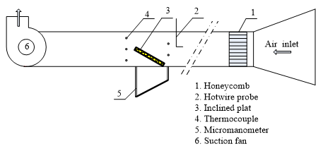
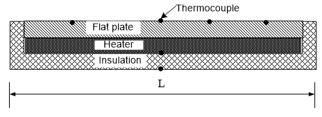
Experiments were performed in a Plexiglas wind tunnel. The experiment test setup mainly consists of a square channel of 30 cm×30 cm, and 50 cm long duct with a suction centrifugal fan, as shown in Figure 1. The fan is rated at 3.67kW and is connected to a variable speed inverter that allows the wind speed to be adjusted. Average airspeeds over the test section ranged from 3.8 m/s to 20 m/s, leading to Reynolds numbers of 67000 and 367000, respectively. The wind speed profile is determined through the duct section using a hot wire anemometer with an accuracy of 0.01 m/s. A flat plate is attached to the test track by a special mechanism that can change the angle of attack. The plate was rotated to alter the angle of attack from 0° to 40° about the vertical axis using a protractor mechanism. The flat plate was heated from below by an electric heater, while, the side opposite the heating element was covered with insulation to reduce heat loss from the other edge of the plate (Figure 2). The decrease in pressure along the plate is assessed using a digital micromanometer with an accuracy of 1 N/m2. The uncertainties for the wind speed and pressure drop measurements are estimated at ±4% and ±1% of the reading, respectively. Velocity and pressure measurements are made as recommended by ASHRAE [23]. Both the horizontal and vertical axes of the plate were fitted with K-type thermocouple probes on a logarithmic scale and the uncertainty was set to 0.5℃. Air temperatures upstream and downstream of the inclined plate were measured with 3- and 6-grid points of K-type thermocouple probes, respectively. A digital thermometer is connected to all thermocouples with a specified level of uncertainty of 0.5℃ through a switch box. The time was sufficient to reach steady state and to obtain a constant modulus measurement experiment, which was observed at about 40-50 min.
Figure 1. Schematic diagram of the test rig
Figure 2. Scheme of the specimen, heater and insulator assembly
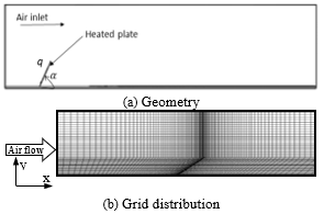
The plate of a length L=25 cm, is heated with a flux, q, and inclined with an angle of attack, α (Figure 3(a)). It is surrounded by air with a velocity similar to the experiment values and even higher. Reynolds number varies from 67000 to 650000. The angle of attack will be varying between 0° and 90°. The flow is incompressible. An inflow limit of three times the length of the plate establishes a uniform flow velocity. At the downstream limit of the plate length, the pressure was set to zero. Constant wall heat flux and no-slip condition are specified on the plate surface. The simulation is two-dimensional, and the results are obtained for steady state regime. The computed domain is given by Figure 3(b).
Figure 3. Problem configuration
The equations describing the thermo-fluid properties of inclined plates are a set of nonlinear PDEs. Airflow is governed by the equations of mass, momentum, and energy. In general, the equations can be written as follows [24, 25]:
Mass:
$\frac{\partial \rho}{\partial t}+\operatorname{div}(\rho \boldsymbol{u})=0$ (1)
Momentum:
$\begin{gathered}\frac{\partial(\rho u)}{\partial t}+\operatorname{div}(\rho u \boldsymbol{u})=-\frac{\partial p}{\partial x}+\operatorname{div}(\mu \operatorname{grad} u)- \left\lceil\frac{\partial \overline{\left(\rho u^{\prime 2}\right)}}{\partial x}+\frac{\partial \overline{\left(\rho u^{\prime} v^{\prime}\right)}}{\partial y}\right\rceil\end{gathered}$ (2)
$\begin{gathered}\frac{\partial(\rho v)}{\partial t}+\operatorname{div}(\rho v \boldsymbol{u})=-\frac{\partial p}{\partial y}+\operatorname{div}(\mu \operatorname{grad} v)- \left\lceil\frac{\partial \overline{\left(\rho u^{\prime} v^{\prime}\right)}}{\partial x}+\frac{\partial\left(\rho v^{\prime 2}\right)}{\partial y}\right\rceil\end{gathered}$ (3)
Energy:
$\frac{\partial(\rho E)}{\partial t}+\operatorname{div}(\rho E \boldsymbol{u})=\operatorname{div}(k \operatorname{grad} T)-\left[\frac{\partial \overline{\left(\rho u^{\prime} E^{\prime}\right)}}{\partial x}+\frac{\partial \overline{\left(\rho v^{\prime} E^{\prime}\right)}}{\partial y}\right]$ (4)
where, u is the velocity vector: u=ux+vy, p is the pressure, μ the fluid viscosity (kg/(m.s)), ρ the fluid density (kg/(m3)), T the temperature (K) and E the energy (J).
As already mentioned in the introduction, there are many turbulence models. As shown by Karava et al. [3], k-ε model is adequate to describe the turbulent flow around the inclined plate. But we decided to use RNG k-ε model because it offers better performance than k-ε by increasing the accuracy and calculating the turbulent Prandtl number, which is more suitable for separation flows [26].
The equations in RNG k-ε model are written as bellow:
$\frac{\partial}{\partial t}(\rho k)+\frac{\partial}{\partial x_i}\left(\rho k u_i\right)=\frac{\partial}{\partial x_i}\left(\alpha_k \mu_{e f f} \frac{\partial k}{\partial x_i}\right)+G_k+G_b-\rho \varepsilon+S_k$ (5)
$\begin{gathered}\frac{\partial}{\partial t}(\rho \varepsilon)+\frac{\partial}{\partial x_i}\left(\rho \varepsilon u_i\right)=\frac{\partial}{\partial x_j}\left(\alpha_{\varepsilon} \mu_{e f f} \frac{\partial \varepsilon}{\partial x_j}\right)+ \\ C_{1 \varepsilon} \frac{\varepsilon}{k}\left(G_k+C_{3 \varepsilon} G_b\right)-C_{2 \varepsilon} \rho \frac{\varepsilon^2}{k}-R_{\varepsilon}+S_k\end{gathered}$ (6)
where, $G_k=-\rho \overline{u_i^{\prime} u_j^{\prime}} \frac{\partial u_j}{\partial x_i}, R_{\varepsilon}=\frac{C_\mu \rho \xi^3\left(1-\xi / \xi_o\right)}{1+\theta \xi^3} \frac{\varepsilon^2}{k}$, $G_b=g_i \frac{\mu_t}{\rho P r_t} \frac{\partial \rho}{\partial x_i}, C_{3 \varepsilon}=\tanh \left|\frac{v}{u}\right|, S_k=\xi \varepsilon$.
The model constants; C1ε, C2ε, ak, ae, ξo and θ in Eqns. (5) and (6) are: C1ε=1.42; C2ε1.68; αεk; ξ=4.34; and θ=0.012, Gk and Gb are turbulent kinetic energy production due to velocity and buoyancy forces, respectively. αk and αε are the reciprocal of (Pr) for both k and ε respectively.
For the energy equation, it becomes as the following:
$\frac{\partial(\rho E)}{\partial t}+\frac{\partial}{\partial x_i}\left(u_i(\rho E+p)\right)=\frac{\partial}{\partial x_j}\left(k_{e f f} \frac{\partial T}{\partial x_j}+u_i\left(\tau_{i j}\right)_{e f f}\right)+S_h$ (7)
where, E is the total energy, $k_{\text {eff }}$ the effective thermal conductivity and $\left(\tau_{i j}\right)_{e f f}$ the deviatoric stress tensor defined:
$\left(\tau_{i j}\right)_{e f f}=\mu_{e f f}\left(\frac{\partial u_j}{\partial x_i}+\frac{\partial u_i}{\partial x_j}\right)-\frac{2}{3} \mu_{e f f} \frac{\partial u_k}{\partial x_k} \delta_{i j}$ (8)
The Eqs. (1)-(8) will be resolved numerically using Ansys Fluent software.
In order to quantify the heat transfer, Nusselt number is determineted. Local Nusselt number is defined as [26]:
$\mathrm{Nu}_{\mathrm{x}}=\frac{q_p X_p}{\left(T_p-T_b\right) K}$ (9)
With qp: heat flux at point p, Xp: location of point p on the plate, Tp: plate temperature, Tb: bulk temperature of the air at point p and K: air thermal conductivity.
Average Nusselt number, Nu, is the mean of local Nusselt number calculated on the plate.
The coefficient of skin friction is also determined using the expression:
$f=\frac{\tau_w}{\rho u_b^2}$ (10)
where, τw is wall shear stress at the point the plate, ρ is fluid density and ub is bulk velocity at the location on the plate. Pressure drag force coefficient is expressed as below:
$C_d=\frac{2 \Delta p}{\rho u_0^2}$ (11)
With $\Delta p$: difference of pressure and u0 the velocity of undistributed air flow.
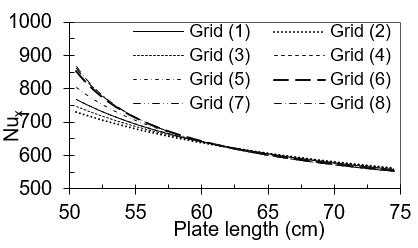
Before investigating the phenomena, a grid dependency study is performed to ensure that the simulation results were independent of the grid density. The number of cells varied from 21300 to 118428 for each computational domain by increasing the cells along X and Y axis. The convergence for some important parameters, such as local and average Nusselt numbers as well as average drag coefficient resulting from pressure, to ensure that the result remains the same regardless of the size of the grid, was achieved. According to Table 1 and Figure 4, Grid (7) is the optimal grid to obtain results similar to very fine grid with less time and CPU memory.
Table 1. Grid sensitivity check for average drag coefficient (Cd) for α=0°, Re=2.74×10⁵ and Pr=0.74
|
Grid |
(∆x, ∆y) |
Number of Cells |
Cd (Average Drag on the Plate) |
|
(1) |
0.50×0.50 |
21300 |
0.00407 |
|
(2) |
0.40×0.40 |
26625 |
0.00400 |
|
(3) |
0.30×0.30 |
35571 |
0.00391 |
|
(4) |
0.25×0.25 |
42600 |
0.00387 |
|
(5) |
0.20×0.20 |
53250 |
0.00384 |
|
(6) |
0.15×0.15 |
70929 |
0.00382 |
|
(7) |
0.10×0.10 |
106500 |
0.00384 |
|
(8) |
0.09×0.09 |
118428 |
0.00382 |
Figure 4. Local Nusselt number in function of plate length for different grids
This research combined experimental and numerical methods to study Reynolds number, heat flux and angle of attack influences on fluid flow and heat transfer properties of the hot plate.
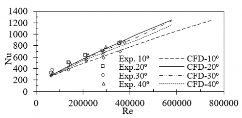
In Figure 5, for q=2000 W/m2, the average Nusselt number (Nu) is presented as a function of Reynolds number (Re) both experimentlly and numerically at α= 0°, 20°, 30° and 40°. For 67000≤Re≤367000, experimental measurements are in good agreement with numerical results with a maximal deviation of 5% that increases sligtly for α=40°. In general, Nu augments when Re increase regardless of α. By increasing the air velocity, the airflow contact becomes higer with the plate which enhances its heating effect. With increasing Re until 370000, Nu at α=20° becomes quite similar to the ones obtained by α=30° and α=40°. Beyond that Re value, Nu at α=20° is the maximal compared to the others.
Figure 5. Experimental and numerical results for Nu vs. Re for q=2000 W/m2 and different angles of attack
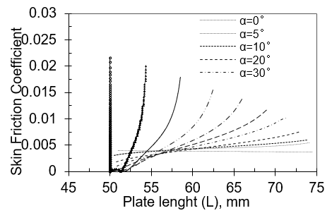
Figure 6. Skin Friction coefficient as function of the plate’s length for Re=2.74×10⁵and different angles of attack
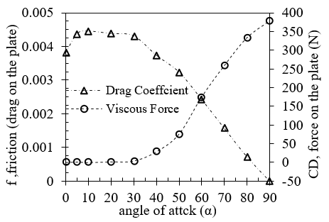
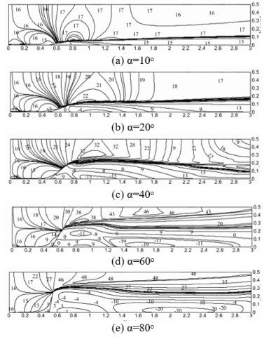
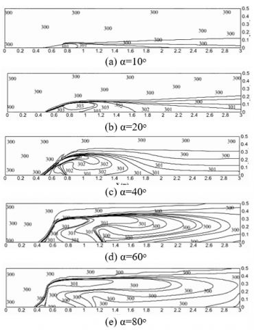
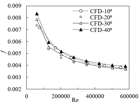
For α=10°, Nu is minimal, especially for very high Re, due to the high skin friction effect noticed from the leading edge of the plate which is greater than the other cases (Figure 6). While for α=20°, skin friction coefficient is low at the leading edge of the plate. Beyond the middle of the plate, the friction becomes more important with the angle increment. With increasing the angle of attack, airflow is hindered due to skin friction resistance. In fact, the drag force is the combination of the skin friction due to viscous force with pressure force. From Figure 7, it is obvious that pressure force is higher than viscous force for low angles of attack, quite similar for α=60° and they switch roles for higher angles with a maximum value of friction at α=90°. This drag force leads to hydrodynamic boundary layer with different thicknesses depending on the chosen angle of attack that generate the turbulent flow on and behind the plate translated by the creation of vortices. Actually, even at the first edge of the plate, a reciculation of air is observed at α=10° (Figure 8), which becomes weaker for high angles. Behind the plate, the airflow is slowed down with the angle increase. This affects the distribution of the temperature in the medium (Figure 9). Whenever the angle is important, the temperature decreases behind the plate. In fact, thermal boundary layer is also playing an important role in either enhancing or decreasing heat transfer. Both hydrodynamic and thermal boundary layers develop at leading edge of the plate and one overcomes the other depending on the plate angle. By increasing Re to very high values, the inclined plate becomes submerged by the turbulent flow, which reduces the skin friction (Figure 10). However, for high angles, the skin friction rises slightly due to the plate resistance over the flow.
Figure 7. Average skin friction and average pressure coefficients for α=0 to 90° and Re=2.74×10⁵
Figure 8. Velocity contours for Re=2.74×10⁵ and different angles of attack
Figure 9. Isotherms for Re=2.74×10⁵ and different angles of attack
Figure 10. Friction factor vs. Reynolds number for q=2000 W/m2 and different angles of attack
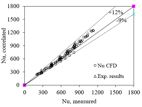
Correlations of average Nusselt number and skin friction coefficient were correlated using both experimental and numerical results for the studied Re range (7.3×10⁴≤Re≤ 5.83×10⁵) and angles of attack (0° to 90°):
$N u=0.186 \operatorname{Re}^{0.664} \operatorname{Pr}^{\frac{1}{3}}\left(0.04 \sin \alpha-0.09 \sin ^2 \alpha\right)$ (12)
with maximum deviations between -9% and 12%, (Figure 11).
$f=0.1985 R e^{-0.314}(1+\sin \alpha)^{0.352}$ (13)
with maximum deviation of ±15%.
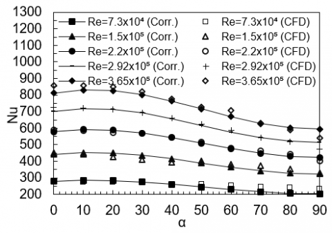
In Figure 12, the average Nusselt number calculated and correlated are plotted as a function of the angle of attack for different Re. A good agreement between the two Nu is observed with a relative difference between the two varying between 0.1% and 12%. For all the plotted Re values, Nu is quite constant for 0°≤α≤30° with a slight increment for α=20° then decreases with α increase. This decrease is more prounounced for high Re. As already explained, the friction is more important when α is high which impacts negatively the circulation of the aiflow and therefore diminish the heat transfer. For 7.19×10⁴≤ Re≤1.5×10⁵ [21], Nu was also found to augment slightly for α≤20°, then decreases beyond α=20°.
Figure 11. Comparison of the present correlation with the present experimental and numerical data
Figure 12. Correlated and numerical average Nusslet number for different angles of attack and Re
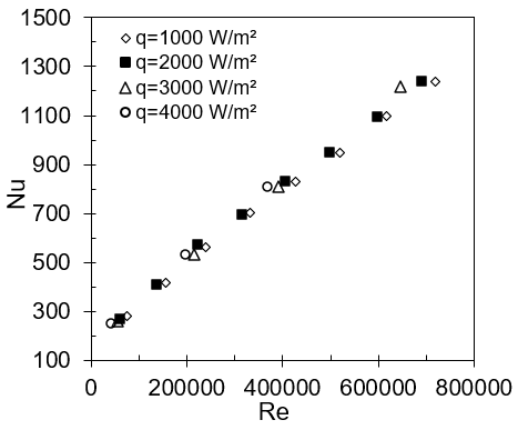
Figure 13. Effect of heat flux on Nusselt number at α=30°
By increasing the heat flux heating the plate (q) from 1000 W/m2 to 4000 W/m2 at α=30°. For Re≤200000, Nu is quite similar for all the heat fluxes. Beyond Re=200000, Nu increases when the heat flux is high, due to the turbulent layer developed that favorites convection circulation, as seen in Figure 13.
Forced convective heat transfer from heated plates for different angles has been investigated experimentally and using Ansys Fluent CFD software. The studied Reynolds numbers range between 72924.6≤Re≤83396.6 and angles of attack range 0°≤α≤40° experimentally, and 0°≤α≤90° numerically. Significant agreement was obtained between the experimental results and the CFD results. The main points of this study are:
Those results can be used to optimize solar panels design to enhance heat transfer and therefore improve their efficiency.
|
CFD |
computational fluid dynamics |
|
f |
friction factor, dimensionless |
|
E |
energy, joule |
|
g |
gravitational acceleration, m.s-2 |
|
grad |
gradient (grad u =$\partial \mathrm{u} / \partial \mathrm{x}+\partial \mathrm{v} / \partial \mathrm{y}$) |
|
h |
Heat transfer coefficient, w.m-2. k-1 |
|
J |
Coulburn factor, dimensionless |
|
k |
thermal conductivity, w.m-1. k-1 |
|
L |
flat plate length, m |
|
Nu |
Nusselt number, dimensionless |
|
Pr |
Prandtl number, dimensionless |
|
∆P |
pressure drop, N/m2 |
|
PDEs |
partial differential equation |
|
Re |
Reynolds number, dimensionless |
|
s |
source term |
|
T |
temperature, K |
|
t |
time, s |
|
u |
velocity vector, (u, v) |
|
u |
air velocity, m/s |
|
x |
x coordinate, m |
|
y |
y coordinate, m |
|
Greek symbols |
|
|
ρ |
density, kg/m3 |
|
$\alpha$ |
thermal diffusivity, m2. s-1 |
|
$\beta$ |
thermal expansion coefficient, k-1 |
|
µ |
dynamic viscosity, kg. m-1.s-1 |
|
κ |
turbulent kinetic energy, m2.s2 |
|
ε |
turbulent dissipation rate, m2.s3 |
|
Subscripts |
|
|
ɸ |
variable |
|
∂ |
rate of change |
|
x |
local distance, m |
[1] Sparrow, E.M., Tien, K.K. (1977). Forced convection heat transfer at an inclined and yawed square plate-application to solar collectors. Journal of Heat Transfer, 99: 507-512. https://doi.org/10.1115/1.3450734
[2] Tari, I., Mehrtash, M. (2013). Natural convection heat transfer from inclined plate-fin heat sinks. International Journal of Heat and Mass Transfer, 56(1-2): 574-593. https://doi.org/10.1016/j.ijheatmasstransfer.2012.08.050
[3] Karava, P., Jubayer, C.M., Savory, E. (2011). Numerical modelling of forced convective heat transfer from the inclined windward roof of an isolated low-rise building with application to photovoltaic/thermal systems. Applied Thermal Engineering, 31(11-12): 1950-1963. https://doi.org/10.1016/j.applthermaleng.2011.02.042
[4] Alshayji, A.E., Ebrahim, S. (2020). Numerical simulation of heat transfer process in inclined roofs with radiant barrier system. Journal of Engineering Research, 8(2): 305-323.
[5] Kumar, D., Premachandran, B. (2022). Investigation of transition in a natural convection flow in an inclined parallel Plate Channel. International Communications in Heat and Mass Transfer, 130: 105768. https://doi.org/10.1016/j.icheatmasstransfer.2021.105768
[6] Jürges, W. (1924). Der Wärmeübergang an einer ebenen Wand Vol. 19: Beiheft zum Gesundheitsingenieur, Druck und R. Oldenbourg Verlag.
[7] Yang, H.Q., Yang, K.T. (1989). Mixed convection from a heated inclined plate in a channel with application to CVD. International Journal of Heat and Mass Transfer, 32(9): 1681-1695. https://doi.org/10.1016/0017-9310(89)90051-3
[8] Siddiqa, S., Asghar, S., Hossain, M.A. (2010). Natural convection flow over an inclined flat plate with internal heat generation and variable viscosity. Mathematical and Computer Modelling, 52(9-10): 1739-1751. https://doi.org/10.1016/j.mcm.2010.07.001
[9] Reda, A. (1989). Air flow and heat transfer characteristics over an inclined flat plate. M. Sc. Thesis, Faculty of Engineering, Cairo University.
[10] Ramirez, C., Murray, D.B., Fitzpatrick, J.A. (2002). Convective heat transfer of an inclined rectangular plate. Experimental Heat Transfer, 15(1): 1-18. https://doi.org/10.1080/089161502753341834
[11] Yang, S.A., Chae, M.S., Chung, B.J. (2020). Natural convection flow separation on the inclined plate depending on inclination and Pr. Transactions of the Korean Nuclear Society Virtual Spring Meeting, July 9-10.
[12] Mahboub, C., Moummi, N., Moummi, A., Youcef-Ali, S. (2011). Effect of the angle of attack on the wind convection coefficient. Solar Energy, 85(5): 776-780. https://doi.org/10.1016/j.solener.2011.01.008
[13] Perovic, B.D., Klimenta, J.L., Tasic, D.S., Peuteman, J.L.G., Klimenta, D.O., Andjelkovic, L.N. (2017). Modelling the effect of the inclinaison angle on natural convection from a plate: The case of a photovoltaic module. Thermal Science, 21(2): 925-938.
[14] Sartori, E. (2006). Convection coefficient equations for forced air flow over flat surfaces. Solar Energy, 80(9): 1063-1071. https://doi.org/10.1016/j.solener.2005.11.001
[15] Cossali, G.E. (2005). Periodic heat transfer by forced laminar boundary layer flow over a semi-infinite flat plate. International Journal of Heat and Mass Transfer, 48(23-24): 4846-4853. https://doi.org/10.1016/j.ijheatmasstransfer.2005.06.005
[16] Vynnycky, M., Kimura, S., Kanev, K., Pop, I. (1998). Forced convection heat transfer from a flat plate: The conjugate problem. International Journal of Heat and Mass Transfer, 41(1): 45-59. https://doi.org/10.1016/S0017-9310(97)00113-0
[17] Shavazi, E.A., Torres, J.F., Hughes, G.O., Pye, J.D. (2018). Convection heat transfer from an inclined narrow flat plate with uniform flux boundary conditions. In Proceedings of the 21st Australasian Fluid Mechanics Conference, Adelaide, Australia.
[18] Sasaki, S., Ashiwake, N. (2002). Enhancement of natural convection heat transfer from an inclined heated plate using rectangular grids. Heat Transfer-Asian Research: Co-sponsored by the Society of Chemical Engineers of Japan and the Heat Transfer Division of ASME, 31(5): 408-419. https://doi.org/10.1002/htj.10043
[19] Lorenzini, G. (2006). Experimental analysis of the air flow field over a hot flat plate. International Journal of Thermal Sciences, 45(8): 774-781. https://doi.org/10.1016/j.ijthermalsci.2005.10.010
[20] Turgut, O., Ozcan, A.C., Turkoglu, H. (2019). Laminar forced convection over an inclined flat plate with unheated starting length. Politeknik Dergisi, 22(1): 53-62. https://doi.org/10.2339/politeknik.403984
[21] El-Shamy, A.R., Sakr, R.Y., Berbish, N.S., Messra, M.H. (2007). Experimental and numerical study of forced convection heat transfer from an inclined heated plate placed beneath a porous medium. In Al-Azhar Engineering Ninth International Conference, Cairo, Egypt.
[22] Adhikari, R.C., Wood, D.H., Pahlevani, M. (2020). An experimental and numerical study of forced convection heat transfer from rectangular fins at low Reynolds numbers. International Journal of Heat and Mass Transfer, 163: 120418. https://doi.org/10.1016/j.ijheatmasstransfer.2020.120418
[23] ASHRAE Handbook of Fundamentals. (2001). SI edition, chapter 14, ASHRAE Inc., Atlanta, GA, USA.
[24] Versteeg, H.K., Malalasesekera W. (1995). An Introduction to Computational Fluid Dynamics, the Finite Volume Method. Longman Group LTD, UK.
[25] Speziale, C.G., Thangam, S. (1992). Analysis of an RNG based turbulence model for separated flows. International Journal of Engineering Science, 30(10): 1379-1388. https://doi.org/10.1016/0020-7225(92)90148-A
[26] FLUENT, 2013 user’s manual, Fluent Inc., USA.