Gianni Martinazzoli*![]() | Benedetta Grassi
| Benedetta Grassi![]() | Daniele Pasinelli | Adriano M. Lezzi
| Daniele Pasinelli | Adriano M. Lezzi![]() | Mariagrazia Pilotelli
| Mariagrazia Pilotelli![]()
(This article is part of the Special Issue 8th AIGE/IIETA International Conference and 18th AIGE Conference)
© 2023 IIETA. This article is published by IIETA and is licensed under the CC BY 4.0 license (http://creativecommons.org/licenses/by/4.0/).
OPEN ACCESS
A primary objective of contemporary district heating (DH) networks is to minimize the use of primary energy, especially fossil fuels, for meeting the heating demands of grid customers. In this context, thermal energy storages (TESs) serve as crucial devices, facilitating the decoupling of grid demand from heat generation. This study presents an experimental comparison of three large-scale TESs, each employing distinct injection and extraction systems. The performance of these were examined based on data collected over a consistent two-month operational period, enabling a quantitative comparison. The TESs under scrutiny, located in the DH networks of Milan and Brescia in Northern Italy, each have a capacity of a few thousand cubic meters of water and differ in their injection system and shape ratio. Notably, the evolution and thickness of the thermocline and the percentage of energy waste were examined to discern the impact of the injection system, specifically the presence of a flow-straightening device, and the shape ratio on the performance of the TES systems. These characteristics were found to significantly influence energy waste in heat storage, which ranged from 1.56% to 6.50% of the total stored energy, depending on the specific TES tank under consideration.
district heating, flow-straightening, TES tank, thermocline, toroidal manifolds
Short-term thermal energy storages (TESs) strategically contribute to the leveling of daily thermal energy demand and counteracting peak heat demand within the district heating (DH) sector. Consequently, they influence the flexibility of the DH network alongside the thermal inertia of buildings and the network itself [1]. The importance of enhancing DH network flexibility via TES units has been underscored in modern DH networks due to the escalating integration of renewable energies and waste heat as replacements for traditional fossil fuel thermal power plants [2]. Moreover, TES units can enhance the utilization of sustainable base load units over peak load units, which are predominantly powered by fossil fuels, thereby reducing CO2 emissions and improving heat generation efficiency [3].
Typically, thermal energy is stored via a storage medium, either through increasing the material's temperature using sensible heat or by leveraging the latent heat associated with the material's phase change. Of the two methods, sensible heat TESs are commercially more viable due to their relatively low cost and ease of operation and maintenance [4]. Indeed, sensible heat TESs are commonly utilized as daily storage in conjunction with DH systems. In particular, TES tanks are filled with the same water as the DH network, serving as a storage medium [5]. These tanks operate based on the stratification of water at different temperatures, with the hot and cold regions separated by the thermocline, a dynamic barrier with a substantial thermal gradient and an intermediate temperature between the hot and cold values, resulting from complex heat transfer by natural convection and gravity forces [6].
Maintaining a high degree of stratification, minimizing the thermocline's thickness, and avoiding mixing effects are vital to achieving maximum storage energy efficiency of the TES. Several performance indicators have been proposed to quantitatively evaluate TES performance, such as exergy efficiency, stratification number, charging and discharging efficiency, and capacity ratio [7]. These performance indicators and the thermocline are significantly influenced by the injection and extraction systems and the tank's shape ratio. The influence of the tank inlet's position on water TES thermal stratification was examined by Li et al. [8], while the impact of the equalizer and diffuser within the TES tank was discussed by Wang et al. [9], Kong and Zhu [10]. The effect of the shape ratio, in particular, is well-documented [11, 12], with better stratification achieved with slim tanks, as demonstrated numerically by Shaikh et al. [12], who found that tanks with a higher shape ratio have better stratification with a smaller thermocline thickness. This result was corroborated by Hosseinnia et al. [13], who found that tanks with a higher shape ratio exhibited superior storage thermal performance. However, these results pertain to water tanks for domestic solar energy storage, and achieving high shape ratio values is not always feasible for large thermal storage tanks such as those for DH due to environmental restriction related to the height of the constructions.
This paper aims to investigate the performance of three TESs, equipped with two different injection and extraction systems and varying capacities and shape ratios. These TESs are integrated into the DH networks managed by the company A2A Calore & Servizi in Milano and Brescia, Northern Italy. The investigation is based on data collected over a two-month winter period with similar daily operation cycles. Experimental analysis on TESs of these sizes – a few thousand cubic meters – is rare in the current literature, as most studies involve smaller tanks used in residential applications and often coupled with thermal solar collectors.
In this paper, a comparison is made between a newer TES, equipped with an innovative injection and extraction system comprising toroidal manifolds and flow-straightening devices, and two older TESs, each composed of two twin tanks without flow-straightening devices and with different toroidal manifold characteristics. The TES tank with the innovative injection system, co-designed by A2A Calore & Servizi and the University of Brescia [14], was installed in the DH network of Brescia and went into operation in January 2020. The system adopted for this tank is the first of its kind, with optimized and experimentally validated perforation characteristics of both the toroidal manifold and the flow-straightening device. A preliminary analysis regarding this TES is reported in the study of Pilotelli et al. [15], while the manifold-only distribution systems adopted in the two older TESs have not yet been experimentally evaluated. These two TESs are integrated into two different DH networks in the Metropolitan City of Milano.
All TESs are equipped with temperature probes, pressure probes, and flow meters necessary to monitor their operation. The Brescia TES has a significantly larger number of probes, specifically designed and installed for the purpose of analyzing the performance of its innovative injection and flow-straightening system. To compare the performance of the two injection systems and determine which solution achieves higher TES efficiency, temperature heat maps displaying the evolution of the measured temperature, graphs illustrating the evolution of the thermocline profile, and some quantitative indicators derived from the available in-field data, have been used. From the measured values, the thermocline thickness, its variation during charging and discharging periods and the consequent percentage of wasted energy have been calculated and compared.
The experimental comparison presented in this paper intends to contribute to the literature on the performance of large-scale TESs and provide quantitative information on the performances of different injection systems. Such information can guide utility companies in choosing the most appropriate solution for new TES tanks.
The manuscript is organized as follows: Section 2 describes the TES tanks and the experimental set-up, and defines the quantitative indicators. Section 3 presents and discusses the obtained results. Section 4 summarizes key conclusions and future directions.
2.1 TES features
All the tanks in the TESs considered in this work are cylindrical atmospheric storages in which the maximum water temperature does not exceed 100℃. Atmospheric TESs are indirectly connected to the DH network, through pumps and valves, due to the pressure difference with the pressurized pipeline of the network.
Two of the analyzed TESs are located in the thermal power plants of Sesto San Giovanni (hereby referred to as “Sesto”) and Canavese, and they serve two DH networks in the Metropolitan City of Milano. Both of them consist of twin tanks, equipped with an injection and extraction system characterized by toroidal perforated manifolds with high-velocity radial injection from the tank wall inwards. The two TESs differ in capacity and shape ratio: the Sesto TES has a total capacity of 4000 m3 provided by two tanks of shape ratio L/D=2.45, while the Canavese TES has a total capacity of 2200 m3 provided by two tanks of shape ratio L/D=1.98.
The third analyzed TES serves the DH network of Brescia, is installed in the “Lamarmora” thermal power plant and is composed of a single tank also equipped with toroidal perforated manifolds with high-velocity radial injection from the tank wall inwards. This TES is more recent than the Sesto and Canavese TESs, and it went into operation in January 2020. The novelty of the Lamarmora injection system, co-designed by A2A Calore & Servizi and the University of Brescia, lies in the perforation of the manifold, which was designed to minimize radial velocity non-uniformity in the circumferential direction, and in the presence of a flow-straightening device consisting of a perforated plate above the lower manifold and one below the upper manifold. The system is described in detail by Pilotelli et al. [14]. The Lamarmora TES has a total capacity of 5500 m3 provided by a single tank of shape ratio L/D=0.94. It is important to notice that with such a low shape ratio careful design of the injection system is crucial to achieve satisfactory performance.
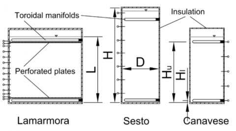
Figure 1 represents the TES tanks analyzed in this study with the main parameters such as the diameter D, the height H, the water level L, the upper toroid height Hu and the lower toroid height Hl. These values are then reported in Table 1 and refer to a single tank of each TES. All the parameters reported in Table 1 are taken from the TES documents made available by the Company A2A Calore & Servizi. Also visible from Figure 1 are the positions of the Pt100 temperature sensors inside the tanks, which are more numerous in the Lamarmora TES with 10 sensors equally spaced 1.5 m along the height of the tank wall, from 1.8 m to 15.3 m, with the addition of a pair of temperature sensors straddling the perforated plates at 0.75-0.97 m and 16.5-16.7 m. On the other hand, in each of the Sesto tanks there are 7 temperature sensors, equally spaced 3.6 m along the height from 2.5 m to 24.1 m, while in each of the Canavese tanks there are 5 temperature sensors, with the lowest sensor at 0.5 m and the others equally spaced by 4 m along the height up to 16.5 m.
Figure 1. Representation at the same scale of the analyzed TES tanks for comparison: The single Lamarmora tank and one of the two identical Sesto tanks and Canavese tanks
Table 1. Main features of the analyzed TES tanks, values refer to a single tank
|
Parameter |
Lamarmora |
Sesto |
Canavese |
|
Nr. tanks |
1 |
2 |
2 |
|
V |
5500 m3 |
2000 m3 |
1100 m3 |
|
D |
19.5 m |
10 m |
9 m |
|
H |
19.7 m |
25.5 m |
19.8 m |
|
L |
17.5-18.5 m |
23.5-24.5 m |
15.8-17.8 m |
|
Hu |
17 m |
22.5 m |
16.5 m |
|
Hl |
0.75 m |
0.6 m |
0.5 m |
|
Nr. Pt100 |
14 |
7 |
5 |
Water temperature and flow rate measurements are also available in the pipes at the inlet and outlet of the tank. For the Sesto and Canavese TESs, consisting of two tanks each, only the total flow rate measurement is available. In the present analysis, it has been assumed that the flow rate is equally distributed between the two tanks. This assumption is justified by the operation of the control system that manages the flow between the two tanks and adjusts the degree of valves opening to distribute the flow evenly. Table 2 and Table 3 show, respectively, the characteristics of the temperature and flow rate sensors for the three TES that were examined.
For TESs connected to DH networks, the temperatures of the hot and cold water coincide with the supply and return temperatures of the DH network, which depend on the characteristics of the network itself. Moreover, the supply temperature can vary during the heating season, reaching higher values in colder periods. As regards the DH network of Brescia, the supply temperature can reach 120℃ near the Lamarmora thermal plant, but the maximum temperature of the water in the Lamarmora TES cannot exceed 99℃ and, if necessary, it is heated further before being fed into the network. The network return temperature is maintained around 60℃, which is the minimum temperature in the TES. As regards the DH networks of Milano to which Sesto and Canavese TESs are connected, the supply temperature is around 90-95℃ and the return temperature around 55-60℃, therefore these temperatures coincide with the maximum and minimum temperatures in the TESs.
Table 2. The main characteristics of temperature probes for different TESs (m.v.: measured value)
|
|
Lamarmora |
Sesto |
Canavese |
|
Sensor type |
Pt 100, 3 wire |
Pt 100, 3 wire |
Pt 100, 3 wire |
|
Range |
0…+150℃ |
0…+150℃ |
0…+150℃ |
|
Maximum error |
± (0.278% m.v.+ 0.20℃) |
± (0.5 % m.v. + 0.3℃) |
± (0.5 % m.v. + 0.3℃) |
Table 3. The main characteristics of flow rate probes for different TESs (m.v.: measured value)
|
|
Lamarmora |
Sesto |
Canavese |
|
Sensor type |
Ultrasonic |
Electromagnetic |
Electromagnetic |
|
Range |
0…2000 m3/h |
0…10 m/s |
0…10 m/s |
|
Maximum error |
± (0.3% m.v. + 2 mm/s) |
± (0.2% m.v.+ 1 mm/s) |
± (0.2% m.v. + 1 mm/s) |
2.2 Comparison methods
The analysis for all TESs is based on data collected during two months, December 2022 and January 2023. The sampling rate for data acquisition is 300s, which is regulated and historicized by the thermal power plants control unit. Specifically, the temperature acquisition systems of Sesto and Canavese TESs only acquires and historicizes a temperature data if it has a difference of more than 1℃ from the previous recorded value. The temperature values measured by the probes at different heights inside the tanks and the flow rate values have been used to compare the performance of the three TESs both qualitatively and by means of a few quantitative parameters, as explained below.
Heat maps. Heat maps are obtained by dividing the height of the tank into a number of layers equal to the number of temperature probes and associating each layer with the value read by the probe, using colors from blue to red for increasing temperatures. The values at different instants of time are represented sequentially, thus a map is obtained that clearly shows the charge and discharge periods and the zones at intermediate temperatures separating the hot and the cold water, i.e., the thermoclines.
Temperature curves. Temperature probes provide temperature evolution over time at the different heights at which they are installed. When a probe detects a temperature change from minimum to maximum, during a charge, or from maximum to minimum during a discharge, it means that the thermocline is crossing it during that time interval. From the flow rate measurements, it is possible to determine the velocity at which water moves vertically during each time interval downward during a charge or upward during a discharge. In the assumption of plug flow, this allows to estimate the displacement of the water mass dx. Therefore, it is possible to plot the read temperature, in abscissa, and the corresponding position within the tank, in ordinate, for each charge and discharge process, for each sensor. These graphs are very useful for visualizing the temperature evolution inside the tank during the charge and discharge cycles. As the thermocline passes through multiple probes in sequence, it is also possible to observe the change in its thickness, as described in the following.
Thermocline thickness. The thermocline is the zone where water is at intermediate temperatures between the maximum and minimum temperatures for the TES – the so-called hot water temperature and cold water temperature. As stated above, for TES connected to a DH network, these temperatures correspond to the supply and return temperatures of the network, which, even in the same network may vary slightly during the heating season. In the present case, they have been set as the maximum temperature (Tmax) and the minimum temperature (Tmin) recorded from the probes in the whole TES during the analyzed two months (97.1℃ and 57.2℃ for Lamarmora; 99.4℃ and 56.3℃ for Sesto; 92.0℃ and 54.9℃ for Canavese). To define the thermocline thickness (htc) , it is necessary to establish its limit temperatures, which in this paper have been determined as a function of the temperature difference between Tmax and Tmin, in accordance with the indication of Zurigat and Ghajar [16]. Therefore, the temperature values identifying the boundary between the hot water and the thermocline ($T_{\text {the,sup }}$) and the cold water and the thermocline ($T_{\text {the,inf }}$) are defined with the following Eqs. (1) and (2).
$T_{\text {the,sup }}=T_{\max }-0.2\left(T_{\max }-T_{\min }\right)$ (1)
$T_{\text {the,inf }}=T_{\min }+0.2\left(T_{\max }-T_{\min }\right)$ (2)
The resulting threshold value are 89.2℃ and 65.2℃ for Lamarmora TES, 90.8℃ and 64.9℃ for Sesto TES and 84.6℃ and 62.3℃ for Canavese TES. The water mass displacement, combined with the temperature readouts, provides the thermocline thickness. Since the temperature values have been recorded at 5-minute time intervals, it is very unlikely that the $T_{\text {the,sup }}$ and $T_{\text {the,inf }}$ are among the measured data: Thus the T(dx) function has been linearly interpolated for the purpose of htc calculation.
Wasted energy. The formation of the thermocline causes the waste of part of the energy introduced into the TES when it is charged with hot water at temperature Tmax: indeed, if the temperature decreases below a certain threshold, it can no longer be fed into the DH network or it may need to be heated further. Thus, in general, a thicker thermocline results in greater wasted energy. In this paper, it has been assumed that the minimum temperature of the water in order to be fed into the DH network is the temperature $T_{\text {the,sup }}$. Therefore, all the energy contained in the thermocline has to be considered wasted.
$E_{\mathrm{was}}=\rho c_p \pi \frac{D^2}{4} \sum_i h_i\left(T_i-T_{\min }\right)$ (3)
where, $\rho$ and $c_p$ are the density and specific heat at constant pressure of water at the mean temperature within the TES, $h_i$ is the thickness of the $i$-th layer, at temperature $T_i$. In addition to the value of $E_{\text {was }}$, it was also evaluated as a percentage of the total energy $E_{\text {tot }}$ that can be charged into the TES tank, determined as
$E_{\text {tot }}=\rho c_p \pi \frac{D^2}{4} L\left(T_{\max }-T_{\min }\right)$ (4)
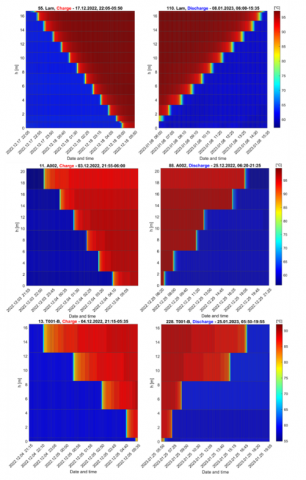
A preliminary qualitative analysis of the transient charge and discharge periods of the three TESs has been carried out by means of heat maps. Example charts are reported in Figure 2, each relating to a complete charge and discharge cycle of the Lamarmora, Sesto and Canavese TESs.
As described in Section 2.2, heat maps illustrate the evolution of the temperature field over time along the height of the tanks, in close relation to the charge and discharge level of the TES. During the charging phase, the temperature increases over time from the top of the TES, due to the hot water that is injected from the upper toroidal manifold, while, at the same time, the cold water is extracted from the lower region of the tank, through the lower toroidal manifold.
On the other hand, in the discharge phase, the temperature inside the TES decreases over time as hot water is extracted from the upper section and supplied to the users, while the return cold water is sent back at the bottom. In these charts, the thermocline can be identified as the layer, or series of layers, between the hot and cold plugs. The different number of sections into which the volume of water in the TES is divided is due to the different number of temperature sensors installed in each tank. In addition, the thickness of the band depends on the distance between two consecutive probes. In this respect, Figure 2 demonstrates the greater availability of measurement points in Lamarmora facility with respect to Sesto and Canavese.
It is worth to noting that, in Figure 2, only 6 layers have been included for Sesto TES instead of 7, which is the actual number of temperature measurement points, because the highest probe is located at an elevation of 24.1 m, but the water level only exceeds this height for 22% of the time for which data are available and when this happens, only by a few centimeters: in fact, the water level covers the probe by at least 10 cm for 12% of the measurement time. For this reason, the temperatures recorded by this probe have been discarded. The problem of the highest probe has not been found in the Lamarmora and Canavese TESs.
From the heat maps selected as the most representative and shown in Figure 2, it can be seen that Lamarmora and Sesto TES appear to have shorter probe temperature transitions and thus lower thermocline thickness values during charge than during discharge. In contrast, Canavese TES shows lower thermocline thickness in discharge than in charge, but with higher values than Lamarmora and Sesto TES.
Figure 2. Charge cycles for Lamarmora TES (top), Sesto TES (middle), and Canavese TES (bottom)
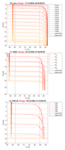
A more accurate study on the behaviour of TES has been carried out by evaluating the evolution of different temperature sensors, from which the thermocline thickness can be derive, as explained in the previous Section. Figure 3 reports the evolution of all temperature sensors within the TES for Lamarmora, Sesto and Canavese in a representative charge cycle. The temperature curves are obtained by linear interpolation between the temperature values measured by the probes, marked by dots. The dashed and dashed-dotted lines indicate the upper and lower limits of the thermocline $T_{\text {the,sup }}$ and $T_{\text {the, inf }}$ respectively, allowing the thermocline thickness to be calculated. The different color shades from red to orange indicate the position of the probes within the TES, from the highest to the lowest.
Figure 3. Evolution of temperature curves over the height for different TES in a charging cycle. From top to bottom: Lamarmora, Sesto and Canavese TES
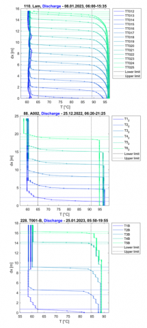
In a similar way, the curves for the discharge cycles have been derived and are shown in Figure 4, again for all the TESs analyzed. In this case, the color shades of the curves range from green, for the highest position of the probe, to blue, for the lowest position.
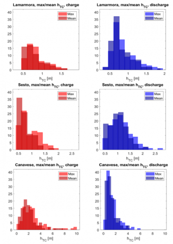
Following the analysis of the evolution of the individual temperature sensors, the average and maximum values of the thermocline thickness have been obtained for each charge and discharge cycle for the two-month period to which the data refer. Figure 5 shows the histograms to represent the number of cycles for which the average thickness and maximum thickness of the thermocline measured in each cycle fall within a given range. The bin width of the histograms is 0.15 m for Lamarmora TES, 0.20 m for Sesto TES, and 0.5 m for Canavese TES.
Figure 4. Evolution of temperature curves over the height for different TES in a discharging cycle. From top to bottom: Lamarmora, Sesto and Canavese TES
From Figure 5 it can be seen that Lamarmora TES and Sesto TES have similar thermocline thickness, with the majority of the distribution between 0.5-1 m for Lamarmora TES and between 0.5-1.5 m for Sesto TES, in the charge cycles. In discharge cycles, the performance of both TES decrease due to the increases in thermocline thickness, which occasionally approaches 2 m for Lamarmora and exceeds 2.5 m for Sesto, but the most of the distribution stays below 1.5 m.
Different values and a different distribution can be observed for Canavese TES, where the largest number of charge cycles has a thermocline thickness up to 4 m, but some cycles reach even higher values, up to 10 m. In contrast to Lamarmora and Sesto TES, the discharge cycles for Canavese TES perform better compared with the charge cycles, and only in one case the thermocline thickness exceeds 4 m.
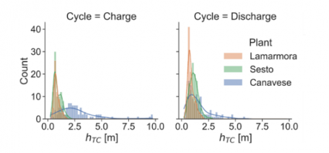
The behavior just described is also visible from Figure 6, which shows, on the same chart, the distribution of the maximum values of the thermocline thickness for the three TESs analysed.
Figure 5. Hystograms showing the number of cycles for which a certain average or maximum thermocline thickness value has been reached, for all TES analysed
For an overall view of the performance comparison of the different TES, the average, the minimum and the maximum value as well as the standard deviation of the thermocline thickness during the analysed period are reported in Table 4 for the Lamarmora, Sesto and Canavese TESs. In particular, the values are given for charge and discharge cycles, which are denoted respectively by the subscript “ch” and “di”. In addition, the global values (i.e., evaluated on all charge and discharge cycles) for all calculated quantities are also given.
The values reported in the Table 4 quantify the trend identified in Figure 5 and Figure 6. Lamarmora and Sesto record a lower thermocline thickness for charging operation than for discharging operation. The opposite situation occurs for the Canavese TES, where the average value of the thermocline thickness increases from discharge to charge cycles. In particular, for Lamarmora TES, which is the only tank equipped with the innovative injection and extraction system, the average thickness of the thermocline is 0.76 m for charging, 0.80 m for discharging, while the overall result is 0.78 m. Values close to Lamarmora are obtained for Sesto TES, in which the global average thickness of the thermocline is 0.86 m (0.71 m in charge and 1.01 m in discharge).
On the other hand, higher values of thermocline thickness result from the Canavese TES, where the globally average value is 1.70 m, reaching 2.15 m in charging and 1.19 m in discharging. As can be seen from Table 4, the highest standard deviation values have been recorded for the Canavese TES for both charge and discharge cycles, with a global value of 1.30 m. Sesto presents a lower standard deviation than Canavese, the global value is 0.36 m. Finally, Lamarmora has the closest thermocline thickness distribution to the average value, with an overall standard deviation of 0.27 m.
Figure 6. Distribution of thermocline thickness for the three TES analysed
Table 4. Minimum, maximum, average and standard deviation of thermocline thickness for the three TESs
|
htc |
Lamarmora |
Sesto |
Canavese |
|
µch [m] |
0.76 |
0.71 |
2.15 |
|
Minch [m] |
0.34 |
0.39 |
0.21 |
|
Maxch [m] |
1.62 |
2 |
9.75 |
|
σch [m] |
0.25 |
0.26 |
1.46 |
|
µdi [m] |
0.80 |
1.01 |
1.19 |
|
Mindi [m] |
0.27 |
0.40 |
0.17 |
|
Maxdi [m] |
1.89 |
2.65 |
5.83 |
|
σdi [m] |
0.29 |
0.38 |
0.83 |
|
µ [m] |
0.78 |
0.86 |
1.70 |
|
Min [m] |
0.27 |
0.39 |
0.17 |
|
Max [m] |
1.89 |
2.65 |
9.75 |
|
σ [m] |
0.27 |
0.36 |
1.30 |
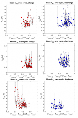
An additional illustration of the average value of the thermocline thickness, along with the maximum and minimum detected ones, is shown in Figure 7. All the quantities in Figure 7 are given as a function of the ratio between the difference of the maximum and minimum temperature registered during a single cycle, and the difference between the maximum and the minimum temperature recorded in the plant during the entire two months for which data are available. From the Figure 7, it can be seen that the values of the thermocline thickness do not depend on the maximum and minimum temperatures recorded in the single cycle, weighed with the absolute maximum and minimum temperatures. However, scaling the temperature difference shows that the dimensionless temperatures recorded in the charge and discharge cycles of Canavese TES are lower compared with those of the Sesto and Lamarmora TESs. Specifically, Lamarmora TES has the highest dimensionless temperature during the operation cycles. Again in relation to the temperatures reached during the charge and discharge cycles at the top and bottom of the tanks, relevant information can be derived from the extreme values of the curves in Figure 3 and Figure 4. In the Lamarmora TES, the different curves tend to collapse between close temperature values, while the same curves in Sesto and Canavese TESs fall in higher temperature ranges. These facts are strongly related with the stirring of water in the top and bottom of the tanks. These stirrings seem to be of lesser magnitude in Lamarmora, allowing higher dimensionless temperature to be maintained. The result appears to be due to the presence of the flow-straightening devices and the careful design and sizing of the toroidal manifold holes that constitute the innovative injection and extraction system. In the case of Canavese, in particular, but also of Sesto, the absence of flow-straightening devices and the different characteristics of the toroidal manifolds cause more significant stirrings, which lead to greater temperature fluctuation at the top and bottom of the TES.
Figure 7. Average, minimum and maximum values of the thermocline thickness. From top to bottom: Lamarmora, Sesto and Canavese TES
It is interesting to observe the relation between the thermocline thickness and the shape ratio of the tanks. The lowest value of thermocline thickness has been obtained for the Lamarmora TES, which is the only one with the innovative injection and extraction system. On the other hand, comparing Sesto and Canavese TESs, neither of which presents the innovative injection and extraction system, Sesto TES records an average thermocline thickness value 0.84 m lower than Canavese. The geometry of Sesto TES is characterised by a shape ratio of 2.45, while the value drops to 1.98 for Canavese TES. Therefore, a remarkable difference in thermocline thickness is likely to be related to the shape ratio. Specifically, when the shape ratio increases, TES performance also improves, according to Shaikh et al. [12] and Hosseinnia et al. [13]. However, the presence of the innovative injection and extraction system is believed to be the reason why in Lamarmora TES the thermocline thickness is contained to 0.78 m despite a low shape ratio of 0.94, very far from the values of the Sesto and Canavese TESs.
Table 5. Wasted energy for different TES in charge
|
Ewas |
Lamarmora |
Sesto |
Canavese |
|
µ [kWh] |
5166 |
1456 |
4023 |
|
µ [%] |
2.07 |
1.54 |
8.41 |
|
Max [kWh] |
10148 |
4721 |
19549 |
|
Max [%] |
4.07 |
5.01 |
40.86 |
|
Min [kWh] |
1816 |
694 |
285 |
|
Min [%] |
0.73 |
0.74 |
0.60 |
Table 6. Wasted energy for different TES in discharge
|
Ewas |
Lamarmora |
Sesto |
Canavese |
|
µ [kWh] |
4999 |
1493 |
2080 |
|
µ [%] |
2.01 |
1.58 |
4.35 |
|
Max [kWh] |
10838 |
6853 |
11693 |
|
Max [%] |
4.35 |
7.27 |
24.44 |
|
Min [kWh] |
1532 |
622 |
203 |
|
Min [%] |
0.61 |
0.66 |
0.43 |
Table 5 and Table 6 show the average, the minimum and the maximum wasted energy both as absolute values and as a percentage of the total energy stored in the three TESs. In particular, Table 5 refers to the charge cycles, while Table 6 to the discharge cycles.
From the two previous tables, Table 7 has been derived, summarising the overall behaviour of the different TESs through the wasted energy as well as providing some features of the geometry and components of the TES. One of the parameters that from the analysis of the results seems to heavily influence the stratification of TES is the shape ratio, expressed in Table 7 as the ratio of the maximum value of water level L to diameter D. Sesto TES has the highest shape ratio and presents the best performance in terms of wasted energy. The Canavese TES has a lower shape ratio than Sesto, with a value of 1.98 instead of 2.45, and its performance decreases, with the global percentage of wasted energy rising from 1.56% for Sesto to 6.50% for Canavese. A different trend is recorded for Lamarmora TES, for which the halving of the shape ratio does not lead to a considerable decrease in TES performance, which is quite close to that of Sesto. Indeed, Lamarmora TES presents a shape ratio of 0.94, but the global percentage of wasted energy is only of 2.04%, instead of 1.56% of Sesto TES.
It is reasonable to assume that this positive result is possible due to the presence of the perforated plates that straighten the flow downstream of the two toroidal manifolds. The presence of the innovative injection and extraction system allows Lamarmora TES to have close performance compared to Sesto in terms of wasted energy, despite the large difference in the shape ratio. Moreover, Lamarmora TES has an even lower thermocline thickness value than Sesto TES. On the other hand, it is noted that the Canavese TES, which is not equipped with the innovative injection system and has a lower shape ratio than Sesto, shows a remarkable decrease in performance with respect to Sesto TES.
Moreover, the innovative injection and extraction system also allows for a more constant thermocline thickness along the height of the TES, as shown in Figure 3 and Figure 4. From these Figures, for Sesto and Canavese TES, it can be seen that the thickness of the thermocline increases in the opposite direction to the direction of flow advance during the transient. Specifically, in the charge cycle (Figure 3), the water flows inside the TES from the top to the bottom and the thermocline thickness increases in the opposite direction, from the lowest to the highest probe. In contrast, in the discharge cycle (Figure 4), water flows from the bottom to the top of the TES and the thermocline thickness always increases in the opposite direction, from the highest to the lowest probe.
The presence of the innovative injection and extraction system in Lamarmora TES does not make this phenomenon evident, with the thermocline thickness not considerably increasing or decreasing in the direction opposite to the flow, but remaining approximately constant. Another positive result, again obtained from the presence of the perforated plates, is the lower standard deviation values of the thermocline thickness of the Lamarmora TES compared to the Sesto and Canavese TESs, demonstrating that the thermocline thickness remains more stable.
Table 7. Wasted energy for different TES
|
|
Lamarmora |
Sesto |
Canavese |
|
Etot |
249 |
94 |
48 |
|
L/D |
0.94 |
2.45 |
1.98 |
|
Innovative injection system |
yes |
no |
no |
|
$\mu\left(E_{\text {was }}\right)[\mathrm{kWh}]$ |
5084 |
1475 |
3109 |
|
$\mu\left(E_{\text {was }}\right)[\%]$ |
2.04 |
1.56 |
6.50 |
It is worth noting that this analysis was performed on data collected during two middle months of the heating season and, for this reason, evaluated as indicative of TES behaviour. The variability of the recorded data is mainly due to the operations of the network that influence the temperature of the supply and return line, which depends on the period of year, the time of day and the heat demand of the users. Moreover, the conclusions drawn may be also influenced by the number of the temperature sensors available for the TESs. The probes within the Sesto tanks are spaced 3.5 m apart each other along the height, similarly in the Canavese tanks the pitch between the probes is 4 m. Therefore, for the Sesto and Canavese TESs, a less detailed description of the temperature evolution along the height of the tank, on which the reconstruction of the thickness of the thermocline is based, is available compared with Lamarmora TES, which features a probe every 1.5 m along height. In addition, as described in Section 2.2, the temperature acquisition systems of Sesto and Canavese TESs only acquires and historicizes a temperature data if it has a difference of more than 1℃ from the previous recorded value. Both of these characteristics lead to the differences between the three analysed TESs that can be observed in Figure 3 and Figure 4. The first characteristic influences the spatial accuracy in the detection of temperatures and the definition of thermocline thickness, while the second justifies the different constant temperature values represented for Sesto and Canavese TESs.
Another factor is the flow split between the two twin tanks that, as described in Section 2.1, constitute the TESs of Sesto and Canavese. In this work, the flow has been assumed to be equally divided between two twin tanks. This assumption is supported by the operation of the control system that manages the degree of valve opening, controlling the flow of water at the inlet of the tanks and theoretically distributing the flow evenly. In reality, the operation system is more complex and related to the operation of the entire DH network. In fact, the TES tanks play another key role inside the network as expansion vessels especially during peaks of heat demand. The DH network is subjected to considerable volumetric expansions and contractions due to the variations in the thermal demand of the grid customers, resulting in different temperature of the supply and return lines over time. To keep this phenomenon under control, TES tanks are also used to support the expansion vessels of the network. Therefore, on one hand, the control system that manages the operation of the TES has a primary regulation on the outflow from the TES that must match the thermal demand or heat generation of the network. On the other hand, the secondary regulation, which manages the flow rate into the tank through the degree of valve opening, is used to control the volumetric expansion of the network. Therefore, the degree of opening of each valve of the two twin tanks is adjusted to counteract volumetric variations and to distribute the flow in order to keep an equal water level within each tank. As a result of the control system, the degree of valve opening is not the same between the twin tanks at all instants of time and they can be considered as two separate tanks. For this reason, a time shift by some minutes in the evolution of the thermocline within the tanks can be observed between the twin tanks in both Sesto and Canavese plants. Especially, the behaviour of the Sesto and Canavese TESs, which show the thermocline thickness growth in the opposite direction from the direction of flow advance within the tank, is difficult to explain physically and is probably due to the unequally instantaneous distribution of the flow between the two tanks, related to the mechanism described in the previous lines.
To counteract the divergence between two separate twin tanks, A2A Calore & Servizi engineered a new flow splitting system and incorporated it in two new twin TES tanks having the same injection and extraction systems as Lamarmora TES, but connected to each other with two pipes, one at the top and the other at the bottom of tank. The double connection between the twin tanks should cancel out the temperature difference of the tanks, allowing the thermodynamic equilibrium to be achieved between the two stored volumes of water. These new twin tanks have been in service in the DH of Brescia since fall 2021 and have not yet been thoroughly analysed to assess their performance.
In the future, these new twin tanks will be compared with the Sesto and Canavese TESs to evaluate the features, components and solutions that enable a large TES to perform better.
This study compares the performance of three large TESs employed in DH networks located in northern Italy and characterized by different shape ratio, capacities, and injection-extraction systems. Specifically, only one of the analyzed TESs, the most recent, is equipped with an innovative injection and extraction system consisting of toroidal manifolds and perforated plates downstream of the manifolds. The analysis is based on data collected during a two-month period in the 2022-2023 heating season. The main parameter chosen to evaluate the performance of TES is the thickness of the thermocline. To compare TESs with different shape ratio and capacities, the thickness of the thermocline has also been converted to a value of wasted energy and compared with the total energy stored in the TES.
From the analysis, it can be seen that the lower thermocline thickness values have been obtained for the TES tank equipped with the innovative injection-extraction systems. Moreover, a decrease in the shape ratio, L/D, leads to a relevant increasing in the thickness of the thermocline for TES that are not equipped of the innovative injection and extraction system. The energy analysis shows how the TES with the lowest level of wasted energy is the one with the highest shape ratio, not equipped with flow-straightening devices. The wasted energy increase considerably, with the decreasing of shape ratio for TES with the same injection and extraction system. Whereas, the increasing in the wasted energy is small for the TES with the innovative injection and extraction system, despite the very low shape ratio.
Therefore, the results show that, in the most recent TES, the presence of the toroidal manifolds having holes designed to minimize radial velocity non-uniformity and the perforated plates exploited as flow-straightening devices contribute to limit and stabilize the thermocline thickness, thus balancing the negative effect of a low shape ratio.
This work constitutes an initial comparison between TESs with different features that will be used in the future as a starting point for comparisons planned for other large TESs recently realized and managed by the company on several DH networks in the northern Italy.
This research was funded by MUR, fund PON “Ricerca e Innovazione” 2014-2020, Azione IV.4 “Dottorati e contratti di ricerca su tematiche dell’innovazione” and Azione IV.5 “Dottorati su tematiche green”.
|
cp |
specific heat at constant pressure, J. kg-1. K-1 |
|
D |
diameter of TES, m |
|
DH |
district heating |
|
E |
energy, J |
|
h |
thermocline thickness, m |
|
H |
height, m |
|
L |
water level, m |
|
T |
temperature, K |
|
TES |
thermal energy storage |
|
V |
volume of TES, m3 |
|
Greek symbols |
|
|
µ |
average |
|
$\rho$ |
water density, kg. m-3 |
|
σ |
standard deviation |
|
Subscripts |
|
|
ch |
charge |
|
cy |
cycle |
|
di |
discharge |
|
i |
i-th layer |
|
l |
lower toroid |
|
max |
maximum |
|
min |
minimum |
|
tc |
thermocline |
|
the, inf |
inferior thermocline boundary |
|
the, sup |
superior thermocline boundary |
|
tot |
total |
|
u |
upper toroid |
|
was |
wasted |
[1] Vandermeulen, A., van der Heijde, B., Helsen, L. (2018). Controlling district heating and cooling networks to unlock flexibility: A review. Energy, 151: 103-115. https://doi.org/10.1016/j.energy.2018.03.034
[2] Lund, H., Werner, S., Wiltshire, R., Svendsen, S., Thorsen, J.E., Hvelplund, F., Mathiesen, B.V. (2014). 4th Generation District Heating (4GDH): Integrating smart thermal grids into future sustainable energy systems. Energy, 68: 1-11. https://doi.org/10.1016/j.energy.2014.02.089
[3] Van Oevelen, T., Scapino, L., Al Koussa, J., Vanhoudt, D. (2021). A case study on using district heating network flexibility for thermal load shifting. Energy Reports, 7: 1-8. https://doi.org/10.1016/j.egyr.2021.09.061
[4] Advaith, S., Parida, D.R., Aswathi, K.T., Dani, N., Chetia, U.K., Chattopadhyay, K., Basu, S. (2021). Experimental investigation on single-medium stratified thermal energy storage system. Renewable Energy, 164: 146-155. https://doi.org/10.1016/J.RENENE.2020.09.092
[5] Guelpa, E., Verda, V. (2019). Thermal energy storage in district heating and cooling systems: A review. Applied Energy, 252: 113474. https://doi.org/10.1016/j.apenergy.2019.113474
[6] Rendall, J., Abu-Heiba, A., Gluesenkamp, K., Nawaz, K., Worek, W., Elatar, A. (2021). Nondimensional convection numbers modeling thermally stratified storage tanks: Richardson's number and hot-water tanks. Renewable and Sustainable Energy Reviews, 150: 111471. https://doi.org/10.1016/J.RSER.2021.111471
[7] Lou, W., Luo, L., Hua, Y., Fan, Y., Du, Z. (2021). A review on the performance indicators and influencing factors for the thermocline thermal energy storage systems. Energies, 14(24): 8384. http://dx.doi.org/10.3390/en14248384
[8] Li, S.H., Zhang, Y.X., Li, Y., Zhang, X.S. (2014). Experimental study of inlet structure on the discharging performance of a solar water storage tank. Energy and Buildings, 70: 490-496. https://doi.org/10.1016/j.enbuild.2013.11.086
[9] Wang, Z., Zhang, H., Dou, B., Huang, H., Wu, W., Wang, Z. (2017). Experimental and numerical research of thermal stratification with a novel inlet in a dynamic hot water storage tank. Renewable Energy, 111: 353-371. https://doi.org/10.1016/j.renene.2017.04.007
[10] Kong, L., Zhu, N. (2016). CFD simulations of thermal stratification heat storage water tank with an inside cylinder with openings. Procedia Engineering, 146: 394-399. https://doi.org/10.1016/j.proeng.2016.06.419
[11] Lavan, Z., Thompson, J. (1977). Experimental study of thermally stratified hot water storage tanks. Solar energy, 19(5): 519-524. https://doi.org/10.1016/0038-092X(77)90108-6
[12] Shaikh, W., Wadegaonkar, A., Kedare, S.B., Bose, M. (2018). Numerical simulation of single media thermocline based storage system. Solar Energy, 174: 207-217. https://doi.org/10.1016/J.SOLENER.2018.08.084
[13] Hosseinnia, S.M., Akbari, H., Sorin, M. (2021). Numerical analysis of thermocline evolution during charging phase in a stratified thermal energy storage tank. Journal of Energy Storage, 40: 102682. https://doi.org/10.1016/J.EST.2021.102682
[14] Pilotelli, M., Grassi, B., Lezzi, A.M., Beretta, G.P. (2022). Flow models of perforated manifolds and plates for the design of a large thermal storage tank for district heating with minimal maldistribution and thermocline growth. Applied Energy, 322: 119436.. https://doi.org/10.1016/j.apenergy.2022.119436
[15] Pilotelli, M., Grassi, B., Pasinelli, D., Lezzi, A.M. (2022). Performance analysis of a large TES system connected to a district heating network in Northern Italy. Energy Reports, 8: 1092-1106. https://doi.org/10.1016/j.egyr.2022.07.094
[16] Zurigat, Y.H., Ghajar, A.J. (2002). Heat transfer and stratification. Thermal Energy Storage: Systems and Applications. http://refhub.elsevier.com/S2352-4847(22)01362-2/sb18.