Mohamed Maniana* | Azzedine Azim | Fouad Errchiqui | Abdelali Tajmouati
© 2022 IIETA. This article is published by IIETA and is licensed under the CC BY 4.0 license (http://creativecommons.org/licenses/by/4.0/).
OPEN ACCESS
The problem posed in the surface heat treatment industry of metallic materials is the knowledge of the amount of energy required and its correct distribution on the treated surface for the achievement of a better quality of the metallurgical structure of treated parts. To succeed in this operation, manufacturers are required to carry out many expensive and time-consuming experiments. This work consists in predicting the energy density applied to the surface of a metal part, during surface heat treatment by a laser beam, based solely on temperature measurements taken under the treated surface. This problem in the mathematical sense is called the reverse heat transfer problem. The solution of this inverse problem of heat conduction allows us to predict the density of the energy necessary to be applied to the surface from the desired metallurgic structure characterized by a well-defined temperature distribution. The optimization method used in this work is that of the conjugate gradient thanks to its speed of convergence, its quality of precision and also to stability. Many similar works have been developed in the literature using the inverse method but only to estimate thermo-physical characteristics such as thermal conductivity, thermal capacity mass, point heat source, etc. using conventional numerical methods. But in no case to estimate the complex profile of an energy density applied to the real processing of steel using the conjugate gradient algorithm.
inverse problem, heat transfer, heat treatment, laser beam, steel, solid-state phase transformation, conjugate gradient method, finite elements method, 3D
Solid-phase heat treatment is applied to the superficial martensitic quenching of low- or non-alloy steels and aims to improve the tribological and mechanical properties of the material (wear, hardness, corrosion, etc.). The purpose of quenching is to modify the microstructure of the steel and cast irons by strengthening the hardness.
The initially ferritic-pearl structure of the material is first austenitized by heating and then transformed into hard martensite by quenching. It is thus possible to carry out a partial or superficial quenching on complex parts and to preserve the greatest ductility of the initial structure of the other areas.
Laser beam quenching is part of the surface quenching process. It is fast, economical, and ecological. It usually uses a continuous OR diode CO2 laser delivering a few kilowatts. This heat treatment process now makes it possible to work on extremely complex geometries, e.g. worm gear camshaft.
Parts treated with laser beam undergo minimal deformations due to the fact that the absorbed laser energy is narrow. Hence the usefulness of the numerical simulation of this heat treatment process is to avoid deformations of the material on the one hand and to predict the final metallurgical structure before doing the experiment on the other hand. And this will make it possible to significantly reduce the cost of manufacturing mechanical parts by reducing the number of experiments and real tests, optimizing the quality of the parts, and controlling energy consumption better.
This physical problem of thermal conduction is modeled in the mathematical sense by an inverse problem.
The first work concerning the solution of the inverse problem was carried out by Stolz [1] in 1960 in the field of aerospace and military. He proposed an analytical solution to the one-dimensional problem obtained by the numerical inversion of the integral equation based on Duhamel's theorem. If one wants to determine the transient flow with good accuracy, it is necessary to take a short time step. The procedure thus proposed then becomes unstable. Indeed, the temperature at an inner point of the solid is damped and out of phase with respect to the surface temperature. In 1962 Beck [2] proposed an approach based on the deconvolution of the inverse problem in the transient and linear case. This method made it possible to adopt a weaker time step.
A technique based on the method of least squares was then presented by Burggraf [3] in 1964. This technique, expressing the surface temperature as a series of temperature and flow derivatives at the measuring point, gives an exact solution to the opposite problem when the data used are known continuously. On the other hand, it becomes approximate when discrete or experimental data are used.
Solving the problems of inverse conduction at the boundaries makes it possible to estimate the parameters (contact thermal resistance, exchange coefficient) and the functions (heat flow density, temperatures) characterizing the heat transfer on an interface.
Knowledge of these parameters or functions is of paramount importance for the numerical simulation of heat transfer within materials. This is why this problem has been the subject of several works in 1D, 2D and see 3D [4-18].
Then come the analytical methods that are based on the principle of superposition or on the Laplace transformation, and are limited to linear problems and simple geometries.
Two other main classes of methods have been developed: function specification methods using criterion minimization and space marching methods in which a subdivision of the field studied is used into two subdomains, one referring to a direct problem and the other identifying with an inverse problem. These include the methods of D’Souza [19], Weber [20], and Hensel Jr and Hills [21], Raynaud and Bransier [22].
The most important criterion for choosing an inverse method is stability. This stability problem can only be solved by the use of the regularization technique. Since the regulation technique cannot be used in inverse methods belonging to the class of return to surface methods.
In 2000, Huang and Chen [23] Used the conjugate gradient method to solve a three-dimensional forced convection inverse problem to estimate heat flow at the surface. In 2002, Kim and Lee [24] developed a solution for the inverse conduction problem using the principle of maximum entropy. In 2007, another solving technique based on the principle of gradient and the resolution of adjoint equations was used by Pujos [25]. In 2008, Lin et al. [26] used the gradient method for solving the inverse problem in forced convection between two parallel plates. In 2010, Lu et al. [27] solved the inverse heat problem in two dimensions to estimate the temperature inside a pipeline. In 2018, El Idi and Karkri [28] have developed heating and cooling conditions effects on the kinetic of phase change of pcm embedded in metal foam.
In other works, the authors have highlighted the influence of temperature on electronic and mechanical equipment Cheng [29], the stresses caused by the friction temperature between cutting tool Niu [30], the influence of fins on heat transfer in parabolic trough solar collectors Badr et al. [31].
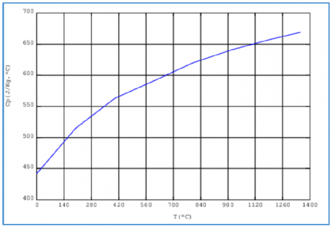
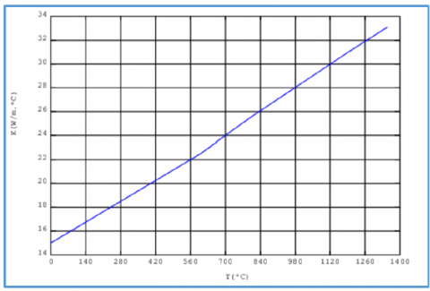
The sample used in this inverse heat transfer problem is a cylindrical part of XC42 heat treatment steel whose geometry is defined on the Table 1. The thermo-physical and metallurgical characteristics of this steel are considered variable with temperature. The temperature-related evolution of these parameters is shown in the Figures 3-5.
The heat treatment of this steel requires the application of two phases:
The search for the heat flow applied to the surface of the cylindrical sample consists in solving three problems:
a- Direct problem using an estimated heat flow $\varphi^n(r, \theta, z, t)$.
b- Adjoint problem by using the error relating to the difference between the measured temperature and the temperature calculated by the direct problem as the energy source.
c- Sensitivity problem using the temperature gradient as a boundary condition.
The results of these three problems allowed us to calculate the depth and decent direction of the conjugate gradient method which will then be used to estimate the new heat flow $\varphi^{n+1}(r, \theta, z, t)$.
2.1 Experiment simulation
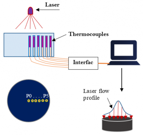
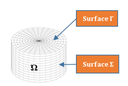
By applying a flow of energy to the heating surface of unknown density, six thermocouples (Figure 1) installed under the surface make it possible to measure the evolution of the temperature Ym(t) at these points, which will be read by the calculation code and serve then to the estimation of the heat flow φ(t), applied to the surface (Γ) (Figure 2), and of the temperature distribution T(t) in the whole calculation domain ( $\Omega$ ) Maniana et al. [32].
Figure 1. Diagram of the experiment
Figure 2. Mesh
2.2 Mesh of the computational domain
For numerical study we have chosen the finite element method a cubic element of 8 nodes an initial density of 0.002 mm, a final density of 0.005 mm and a time step of 0.1 s.
All data necessary for numerical calculation are classified into three categories and defined in Tables 1-3.
Table 1. Sample geometry
|
Quantity |
Value |
|
Diameter [mm] |
100 |
|
Height [mm] |
60 |
|
Mass [kg] |
0.918 |
Table 2. Chemical composition
|
XC42 STEEL |
||||
|
C |
S |
Mn |
P |
Si |
|
0.37 at 0.44 |
0.035 max |
0.50 at 0.80 |
0.035 max |
0.40 max |
Table 3. Mechanical characteristics of XC42
|
Young's Modulus E [GPa] |
Poisson Coefficient ν |
Sigma σ[MPa] |
Reference temperature T ℃ |
|
200 |
0.278 |
230 |
20 |
|
185 |
0.288 |
184 |
200 |
|
170 |
0.298 |
132 |
400 |
|
153 |
0.313 |
105 |
600 |
|
135 |
0.327 |
77 |
800 |
|
96 |
0.342 |
50 |
1000 |
|
50 |
0.350 |
20 |
1200 |
|
10 |
0.351 |
10 |
1340 |
Let us define the heat transfer problems to be solved with the conjugate gradient method as well as the boundary conditions imposed on the boundaries of the computational domain.
4.1 The direct problem
This problem consists in finding the distribution of the temperature in the mass of the sample knowing the density of the heat flow φ applied to the base surface of the cylinder and the evolution of the volume source $\dot{q}$. The heat Eq. (1) is obtained by recording the conservation of thermal energy in an element of volume (V) of any solid:
$\rho c_p \frac{\partial T(r, \theta, z, t)}{\partial t}+\operatorname{div}(-k(T) \cdot \overrightarrow{\operatorname{grad}} T(r, \theta, z, t))=$
$\dot{q}(r, \theta, z, t) \quad$ in $\Omega$ (1)
$-\left.k(T) \frac{\partial T(t, r, \theta, z)}{\partial n_1}\right|_{z=l}=\varphi(r, \theta, z, t)$ on $\Gamma$ (2)
$-\left.k(T) \frac{\partial T(r, \theta, z, t)}{\partial n_2}\right|_{r=R}=h \cdot\left(T(r, \theta, z, t)-T_{\infty}\right)$ on $\Sigma$ (3)
$T(r, \theta, z, t)=T_0$ in $\Omega \quad$ at $t=0$ (4)
After solving the direct problem, we have to calculate the error E(r,θ,z,t) defined by the Eq. (5). This error will serve us as a volume source applied in the Eq. (6) of the adjoint problem defined below.
$E(r, \theta, z, t)=\sum_{n=1}^{N c}\left(T(r, \theta, z, t)-Y_m(t)\right) \delta(r$$\left.-r_m\right) \delta\left(\theta-\theta_m\right) \delta\left(z-z_m\right)$ (5)
4.2 Adjoint problem
Solving this problem will allow us to determine the temperature gradient at the surface Γ.
$\rho(T) c_p(T) \frac{\partial \psi(r, \theta, z, t)}{\partial t}+k(T) \Delta \psi=$ $E\left(r_m, \theta_m, z_m, t, \varphi\right)-\frac{\partial \dot{q}}{\partial T} \psi \quad$ in $\Omega$ (6)
$k(T) \frac{\partial \psi(r, \theta, z, t)}{\partial n_1}=0 \quad$ on $\Gamma$ (7)
$k(T) \frac{\partial \psi(r, \theta, z, t)}{\partial n_2}=0 \quad$ on $\Sigma$ (8)
$\psi(r, \theta, z, t)=0$ in $\Omega \quad$ at $t=t_f$ (9)
The extraction of the solution ψ(r,θ,z,t) of this problem added to the boundary surface Γ will allow us to deduce the gradient and the direction of descent of the conjugate gradient method.
$J^{\prime}\left(\varphi^n\right)=\psi(r, \theta, l, t)$ (10)
$\beta^n=\frac{\left\|J^{\prime}\left(\varphi^n\quad\right)\right\|}{\left\|J^{\prime}\left(\varphi^{n-1}\quad\right)\right\|}$ (11)
$d^n=J^{\prime}\left(\varphi^n\right)+\beta^n d^{n-1}$ (12)
The value of the descent direction will be applied as the heat flow to the heating surface in the following problem. Solving this sensitivity problem will allow us to calculate the depth of descent for the conjugate gradient method.
4.3 Sensitivity problem
In this sensitivity problem we solve the heat Eq. (13), in which we apply as a boundary condition Eq. (14) on the control surface (Г) the heat flow $\delta \varphi$.
$\frac{\partial\left(\rho c_p(T) \delta T(r, \theta, z, t)\right)}{\partial t}-\Delta(k(T) \delta T(r, \theta, z, t))=$$\frac{\partial \dot{q}}{\partial T} \delta T(r, \theta, z, t) \quad$ in $\Omega$ (13)
We set: $\delta \varphi=d^n$
$\frac{\partial(k(T) \delta T(r, \theta, z, t))}{\partial n_1}=\delta \varphi \quad$ on $\Gamma$ (14)
$\frac{\partial(k(T) \delta T(r, \theta, z, t))}{\partial n_2}=0 \quad$ on $\Sigma$ (15)
$\delta T(r, \theta, z, t)=0$ in $\Omega$ at $t=0$ (16)
The analytical expression for the depth of descent is given by the Eq. (17).
$\gamma=\frac{\int_0^{t_f \sum_{m=1}^{m=N c}\left(T\left(r_m, \theta_m, z_m, t, \varphi\right)-Y_m(t)\right) \delta T\left(r_m, \theta_m, z_m, t, \delta \varphi\right) d t}}{\int_0^{t_f} \sum_{m=1}^{m=N c}\left(\delta T\left(r_m, \theta_m, z_m, t, \delta \varphi\right)\right)^2 d t}$ (17)
The estimate of the new heat flow sought is given by the following relationship:
$\varphi^{n+1}=\varphi^n-\gamma^n d^n$ (18)
The convergence condition is imposed by the minimization of the functional defined below:
$J\left(\varphi^n\right)=\sum_{m=1}^{m=N_c}\left[T_m\left(\varphi^n\right)-Y_m\left(\varphi^n\right)\right]^2$ (19)
4.4 Algorithm of this conjugate gradient method
This algorithm shows the hierarchy to follow in the conjugate gradient method to determine the new flux $\left(\varphi^n\right)$ from the estimated flow $\left(\varphi^{n-1}\right)$ in the previous step.
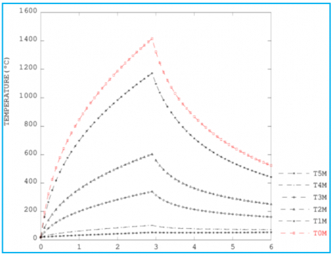
In the Figure 6 we represent the evolution of the temperature versus time in the six measurement points obtained by experimental simulation.
In the Figure 7 we represent in 3D the mapping of the applied flow to the heated surface, obtained by numerical calculation.
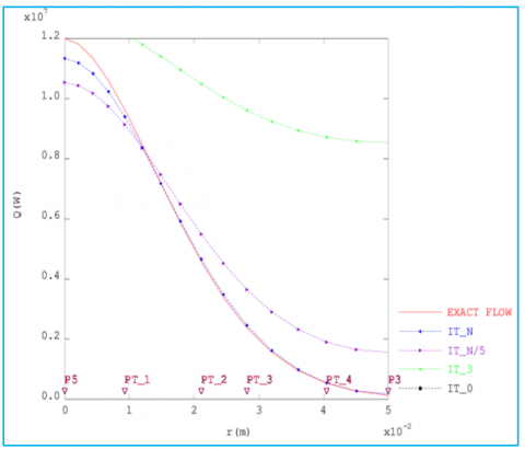
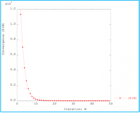
The Figure 8 represents the convergence of the estimated heat flow, depending on the number of iterations (N), towards the exact solution.
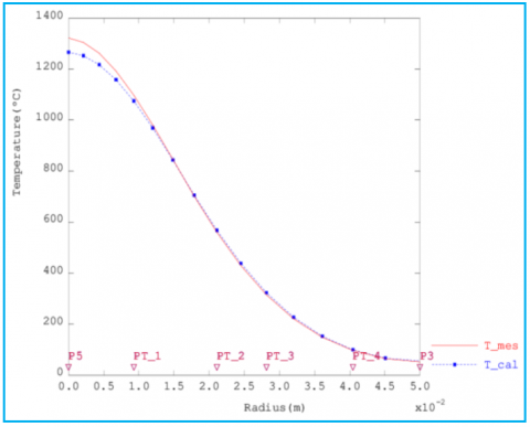
In Figure 9 we compared the radial profile of the temperature obtained by the numerical method with the profile estimated experimental.
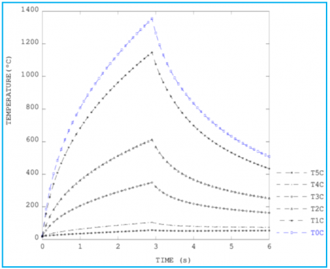
In Figure 10 we represent the evolution versus time of the temperature in the six measurement points, obtained by the numerical method.
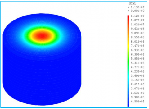
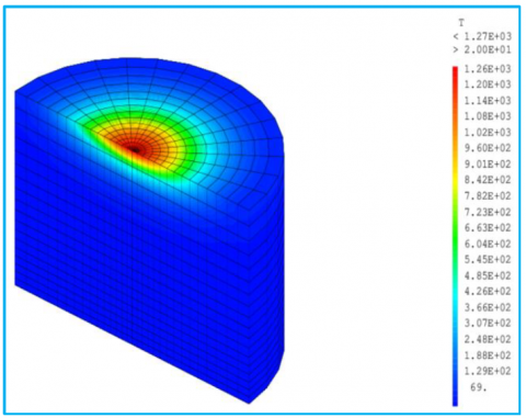
The Figure 11 represents the temperature map in half of the sample at the end of the heating phase.
The Figure 12 shows the rapid evolution of the convergence criterion versus the number of iterations.
In Figure 13 we have made a comparison between the calculated temperature and that measured at the measurement point pt_0, located in the center of the heated surface of the sample.
Figure 6. Measured temperature
Figure 7. Applied flow
Figure 8. Heat flow iteration
Figure 9. Measured and calculated temperature profile at index point (P0)
Figure 10. Calculated temperature profile
Figure 11. Temperature distribution in the sample
Figure 12. Convergence criterion
Figure 13. Comparison of T0C and T0M
By the comparison between the measured temperature, at the center of the heated surface, and that calculated by the numerical method at the same geometric point, we found that the conjugate gradient method converges quickly and efficiently towards the exact solution.
The limitation of this technique of evaluating the thermal source by the inverse method is summarized in the efficiency of access to temperature measurement inside the material.
The prospect of this work is to make a thermomechanical coupling in order to be able to make a complete study of the behaviour of the material from the point of view of deformations and structure after surface treatment.
|
$\emptyset$ |
Heat flow (W) |
|
φ |
Surface heat flow (W.m-2) |
|
k |
Conductivity (W.m-1.K-1) |
|
ρ |
Density (kg.m-3) |
|
cp |
Mass calorific capacity (mass heat) (J.kg-1.K1) |
|
h |
Convection coefficient (W.m-2.K-1) |
|
t |
Time (s) |
|
tf |
final time (s) |
|
q |
Volumetric Heat Flow (W.m-3) |
|
r |
Contact Radius (m) |
|
S |
Surface (m²) |
|
T |
Temperature (°C) |
[1] Stolz Jr, G. (1960). Numerical solutions to an inverse problem of heat conduction for simple shapes. Journal of Heat Transfer, 82: 20-26. https://doi.org/10.1115/1.3679871
[2] Beck, J.V. (1968). Surface heat flux determination using an integral method. Nuclear Engineering and Design, 7(2): 170-178. https://doi.org/10.1016/0029-5493(68)90058-7
[3] Burrgraf, O.R. (1964). An exact solution of the inverse problem in heat conduction, theory and application. Journal of Heat Transfer, 86: 381-382. https://doi.org/10.1115/1.3688702
[4] Al-Khalidy, N. (1998). A general space marching algorithm for the solution of two-dimensional boundary inverse heat conduction problems. Numerical Heat Transfer, Part B, 34(3): 339-360. https://doi.org/10.1080/10407799808915062
[5] Bogatin, O., Chersky, I., Starostin, N. (1993). Simulation and identification of nonstationary heat transfer in a nonuniform friction contact. Journal of tribology, 115: 299-306. https://doi.org/10.1115/1.2921006
[6] Huang, C.H., Tsai, C.C. (1998). A transient inverse two-dimensional geometry problem in estimating time-dependent irregular boundary configurations. International Journal of Heat and Mass Transfer, 41(12): 1707-1718. https://doi.org/10.1016/S0017-9310(97)00266-4
[7] Hao, D.N., Reinhardt, H.J. (1995). Stable numerical solution to linear inverse heat conduction problems by the conjugate gradient method. Journal of Inverse and Ill-posed Problems, 3: 447-467. https://doi.org/10.1515/jiip.1995.3.6.447
[8] Tseng, A.A., Zhao, F.Z. (1996). Multidimensional inverse transient heat conduction problems by direct sensitivity coefficient method using a finite-element scheme. Numerical Heat Transfer, 29(3): 365-380. https://doi.org/10.1080/10407799608914987
[9] Maillet, D., Degiovanni, A., Pasquetti, R. (1991). Inverse heat conduction applied to the measurement of heat transfer coefficient on a cylinder: Comparison between an analytical and a boundary element technique. Journal of heat Transfer, 113: 549-557. https://doi.org/10.1115/1.2910601
[10] Martin, T.J., Dulikravich, G.S. (1998). Inverse determination of steady heat convection coefficient distributions. Journal of heat Transfer, 120: 328-334. https://doi.org/10.1115/1.2824251
[11] Park, H.M., Chung, O.Y., Lee, J.H. (1999). On the solution of inverse heat transfer problem using the Karhunen–Loeve Galerkin method. International Journal of Heat and Mass Transfer, 42(1): 127-142. https://doi.org/10.1016/S0017-9310(98)00136-7
[12] Peneau, S., Humeau, J.P., Jarny, Y. (1996). Front motion and convective heat flux determination in a phase change process. Inverse Problems in Engineering, 4(1): 53-91. https://doi.org/10.1080/174159796088027633
[13] Tseng, A.A., Zhao, F.Z. (1996). Multidimensional inverse transient heat conduction problems by direct sensitivity coefficient method using a finite-element scheme. Numerical Heat Transfer, 29(3): 365-380. https://doi.org/10.1080/10407799608914987
[14] Tortorelli, D.A., Michaleris, P. (1994). Design sensitivity analysis: overview and review. Inverse problems in Engineering, 1(1): 71-105. https://doi.org/10.1080/174159794088027573
[15] Truffart, B. (1996). Méthode d'optimisation pour la résolution de problèmes inverses de conduction de la chaleur (Doctoral dissertation, Nantes).
[16] Lair, P., Dumoulin, J., Bernhart, G., Millan, P. (1997). Etude numérique et expérimentale de la résistance thermique de contact à hautes températures et pressions élevées. In SFT 97-Congrès annuel de la Société Française des Thermiciens, 5: 199.
[17] Reulet, P., Dumoulin, J., Millan, P. (1997). Identification du coefficient de transfert de chaleur pariétal instationnaire. Congrée SFT97, Toulouse, France, 20-22.
[18] Reulet, P., Escriva, X., Marchand, M., Giovannini, A., Millan, P. (1997). Etude locale instationnaire des coefficients d’échanges pariétaux pour des interactions tourbillon-paroi. Congrèes SFT97, Toulouse, France, 20-22. https://doi.org/10.1016/S0035-3159(98)80044-5
[19] D’Souza, N. (1973). Inverse heat conduction problem for prediction of surface temperatures and heat transfer from interior temperature measurements, Report No. SRC-R-74 Space research Corporation, Montreal, December 1973.
[20] Weber, C.F. (1981). Analysis and solution of the ill-posed inverse heat conduction problem. International Journal of Heat and Mass Transfer, 24(11): 1783-1792. https://doi.org/10.1016/0017-9310(81)90144-7
[21] Hensel Jr, E.C., Hills, R.G. (1984). A space marching finite difference algorithm for the one dimensional inverse conduction heat transfer problem. In National Heat Transfer Conference.
[22] Raynaud, M., Bransier, J. (1986). A new finite difference methode for nonlinear inverse heat conduction problem. Numerical heat transfer, 9(1): 27-42. https://doi.org/10.1080/10407788608913463
[23] Huang, C.H., Chen, W.C. (2000). A three-dimensional inverse forced convection problem in estimating surface heat flux by conjugate gradient method. International Journal of Heat and Mass Transfer, 43(17): 3171-3181. https://doi.org/10.1016/S0017-9310(99)00330-0
[24] Kim, S.K., Lee, W.I. (2002). Solution of inverse heat conduction problems using maximum entropy method. International Journal of Heat and Mass Transfer, 45(2): 381-391. https://doi.org/10.1080/716100491
[25] Pujos, C. (2007). Influence des incertitudes paramétriques sur l’estimation d’un modèle rhéologique par inversion de mesures de débit et de températures. 18ème Congrès Français de Mécanique, Grenoble (France), 27-31 aout 2007.
[26] Lin, D.T., Yan, W.M., Li, H.Y. (2008). Inverse problem of unsteady conjugated forced convection in parallel plate channels. International Journal of Heat and Mass Transfer, 51(5-6): 993-1002. https://doi.org/10.1016/j.ijheatmasstransfer.2007.05.022
[27] Lu, T., Liu, B., Jiang, P.X., Zhang, Y.W., Li, H. (2010). A two-dimensional inverse heat conduction problem in estimating the fluid temperature in a pipeline. Applied Thermal Engineering, 30(13): 1574-1579. https://doi.org/10.1016/j.applthermaleng.2010.03.011
[28] El Idi, M.M., Karkri, M. (2020). Heating and cooling conditions effects on the kinetic of phase change of PCM embedded in metal foam. Case Studies in Thermal Engineering, 21: 100716. https://doi.org/10.1016/j.csite.2020.100716.
[29] Cheng, Y. (2022). Thermal fault detection and severity analysis of mechanical and electrical automation equipment. International Journal of Heat and Technology, 40(2): 604-610. https://doi.org/10.18280/ijht.400230
[30] Niu, M. (2022). Stress of ZrN-Coated cutting tools under high temperature friction. International Journal of Heat and Technology, 40(2): 482-488. https://doi.org/10.18280/ijht.400216
[31] Badr, M.K., Ali, F.H., Sheikholeslami, M. (2022). Influence of internal fins and nanoparticles on heat transfer enhancement through a parabolic trough solar collector. International Journal of Heat and Technology, 40(2): 436-448. https://doi.org/10.18280/ijht.400211
[32] Maniana, M., Azim, A., Rhanim, H., Archambault, P. (2009). Problème inverse pour le traitement laser des métaux à transformations de phases. International Journal of Thermal Sciences, 48(4): 795-804. https://doi.org/10.1016/j.ijthermalsci.2008.05.018