Xiaolong Cheng* | Xujin Zhang | Jun Wu
© 2022 IIETA. This article is published by IIETA and is licensed under the CC BY 4.0 license (http://creativecommons.org/licenses/by/4.0/).
OPEN ACCESS
Compared with traditional low-standard ship locks, large-section navigable tunnels have the advantages of increasing water resources dispatching, increasing ship crossing channels and shipping. It is necessary to explore the characteristics of navigable flow conditions under the condition of navigable tunnel and study effective measures to improve the navigable flow conditions at the entrance of approach channel of navigable tunnel in steep bay section. However, the existing research results neglect the navigation channel layout in the steep bay section, and it’s lack of theoretical research on improving the flow conditions at the entrance of approach channel of navigable tunnel in the steep bay section. For this, this article studies the characteristics of navigation flow conditions and numerical simulation of water conservancy in steep bay section of the tunnel. Firstly, the physical model of tunnel navigation in steep bay section is designed to ensure the geometric similarity, flow movement similarity and dynamic similarity between the model and the actual situation in steep bay section. Then, the numerical simulation of navigation water conservancy in steep bay section of tunnel is carried out, and the continuity equation and momentum equation in the new coordinate system are given. This article explores the navigation scheme of large cross-section navigable tunnel in order to obtain effective measures to improve the navigation conditions of this section. Finally, the corresponding experimental results and analysis are given.
steep bay, navigable tunnel, analysis of flow condition characteristics, numerical simulation of water conservancy
With the rapid development of China's economy and the increasing demand for inland navigation, China faces the gradually increasing navigation pressure, and more and more special navigation channel construction schemes are put on the agenda to solve the outstanding shipping problem of low efficiency of crossing gates [1-12]. Compared with the traditional low-standard ship locks, the large-section navigable tunnel has the advantages of increasing water resources dispatching, increasing ship crossing channels and shipping [13-16].
Navigable tunnels are usually set in curved rivers with complex flow patterns and uneven velocity distribution. Because the navigable flow in restricted waters has the characteristics of high wave and rapid velocity, the navigation process of ships is vulnerable to have many adverse effects on the buildings and facilities on both sides of the river, the sediment of rivers and its own navigation stability [17-21]. Therefore, it is necessary to explore the characteristics of navigable flow conditions under the condition of navigable tunnel and study effective measures to improve the navigable flow conditions at the entrance of approach channel of navigable tunnel in steep bay section.
In order to fill in the blank of the research on the key technologies of ship navigation safety in navigable tunnels, the study of Deng et al. [22] establishes a numerical model based on FUNWWAVE-TVD, an open source software package of completely nonlinear Boussinesq equation, to demonstrate the traveling wave motion of ships in navigable tunnels in linear canals. This study provides a reference and basis for the design of single-track straight channel navigable tunnel, and provides a theoretical basis for formulating any key technical standards or specifications for ship navigation safety in navigable tunnel. Based on the typical riverbed topography and hydrodynamic conditions, combined with the layout of the exit guide wall of Babao Ship Lock and the construction scheme of three tidal gates, Yang et al. [23] calculated the plane flow pattern in the exit channel area. In addition, it uses the variation of plane flow field at typical local time outside the entrance area, the size of backflow region, the lateral velocity and longitudinal velocity in the entrance channel to analyze and compare the navigation flow conditions of different schemes. Böttner et al. [24] carried out physical model tests, and designs and constructs a scale model (1:40) to carry two laser Doppler velocimetry sensors and provide optical channels at different positions of the hull to detect the water flow near the bottom of the hull and solve the boundary laminar flow at the hull. Wu and Ding [25] established the physical model of Jiaogang Shiplock. Through model test, the flow situation of lock chamber and approach channel is studied. The results show that when the upstream water level remains high and the difference between upstream and downstream water levels is less than 0.5 m, the annual spring tide discharge and mainstream oscillation during backflow are small.
Scholars at home and abroad have carried out a large number of studies on the flow movement law in the sharp bay section, including the analysis of flow velocity distribution and resistance distribution in the sharp bay section by means of observation, flume test and solid generalized model. However, the existing research results neglect the navigation channel layout in the steep bay section, and it’s lack of theoretical research on improving the flow conditions at the entrance of approach channel of navigable tunnel in the steep bay section. For this, this article studies the characteristics of navigation flow conditions and numerical simulation of water conservancy in steep bay section of tunnel. Firstly, in the second chapter, the physical model of tunnel navigation in steep bay section is designed to ensure the geometric similarity, flow movement similarity and dynamic similarity between the model and the actual situation in steep bay section. Then, in the third chapter, the numerical simulation of navigation water conservancy in steep bay section of tunnel is carried out, and the continuity equation and momentum equation in the new coordinate system are given. The fourth chapter explores the navigation scheme of large cross-section navigable tunnel in order to obtain effective measures to improve the navigation conditions of this section. Finally, the corresponding experimental results and analysis are given.
Constrained by boundary conditions such as topography, the flow conditions in the steep bay section are more complex, and the flow conditions in the entrance area of the approach channel of the navigable tunnel in the steep bay section affected by oblique flow at the head of the diversion dike and discharge from the sluice gate will be more complex. In this article, the Shipai Project between the Three Gorges Dam is taken as the main research object, and the navigable flow conditions in the entrance area of the approach channel of the lower navigable tunnel in steep bay section are studied in detail.
From the aerial photography of the Yangtze River on the south side of Shipai, it can be clearly seen that the Yangtze River is just in Shipai, turning a very hard bend to the right, and showing a sharp bay of 90 degrees. If you look at the latest map of China, this bend lies between the Three Gorges Dam and Gezhouba Dam. Sixty years ago, the rushing Three Gorges was still the most convenient passage into Sichuan, and Shipai was just waiting at the easternmost end of this passage. The riverbed elevation drops and rises steeply, the width of the river reach is about 345m, the curvature radius of the bend is about 750m, and the water depth is about 90m, so it is difficult to implement the general regulation measures. At the same time, the river surface of steep bay section in Shipai reach is narrow in flood season, which has the problem of insufficient hub layout width. At the same time, due to the influence of bend flow and trajectory-bucket flow, the navigation flow conditions are poor, which will make it difficult for upstream and downstream ships to enter and exit the approach channel, and the risk of safe navigation is huge.
In order to put forward new regulation measures to improve the navigable flow conditions in this section, it is necessary to comprehensively consider the river regime conditions in this area and the setting requirements of water control projects, further explore the characteristics of water flow conditions in the entrance area of approach channel under different navigation schemes, and accurately judge whether the water flow conditions under this scheme meet the requirements of safe navigation of ships.
According to the research purpose and the requirements of physical model experiment and based on the actual conditions of navigable channel characteristics, riverbed morphology and topography in the steep bay section, the physical model constructed is determined as a 1:100-scale integral fixed bed normal model. The model design needs to abide by the gravity similarity criterion and ensure the geometric similarity, flow movement similarity and dynamic similarity between the model and the actual situation in the steep bay section.
Geometric similarity is to ensure that the spatially corresponding size ratio between the constructed physical model and the actual situation of navigation at the approach channel entrance area of the navigation tunnel is constant. Assuming that the plane scale is represented by μK, the vertical scale is represented by μF, the actual length of the sharp bay section is represented by KE, and the model length is represented by Kn, then:
${{\mu }_{K}}={{\mu }_{F}}=\frac{{{K}_{e}}}{{{K}_{n}}}$ (1)
Flow movement similarity means that the physical model constructed is geometrically similar to the navigable flow velocity field in the entrance area of the approach channel of the navigable tunnel. Assuming that the velocity scale is expressed by μu, then:
${{\mu }_{u}}={{\mu }_{K}}^{\frac{1}{2}}$ (2)
Dynamic similarity means that all the forces at the corresponding points of the physical model constructed and the entrance area of the approach channel of the navigable tunnel are parallel to each other and the magnitude ratio is constant. Assuming that the forces acting on the corresponding points in the entrance area of the approach channel of the navigable tunnel are represented by GE and the forces acting on the model are represented by GN, then:
${{\mu }_{G}}={{G}_{e}}/{{G}_{N}}$ (3)
In addition to the above three similarities, the normal fixed bed model also needs to meet a series of limiting conditions. Assuming that the flow resistance coefficient is expressed by ge, ge=2hm2/s1/3e, the following equation gives the inequality of the limiting conditions of the resistance square region:
${{\mu }_{F}}\le 4.22{{\left( \frac{{{U}_{E}}{{F}_{E}}}{\alpha } \right)}^{2/11}}g_{E}^{8/11}\mu _{K}^{8/11}$ (4)
Turbulence limiting conditions are given by the following formula:
$S{{p}_{m}}=\frac{US}{u}\ge 1000$ (5)
The mathematical model has the advantages of short experimental period, no scaling effect and high simulation efficiency. Furthermore, based on the DELFT3D model, this article establishes the navigable flow model in the entrance area of the approach channel of the navigable tunnel in steep bay section, studies its flow characteristics, and makes a detailed study on how to improve its flow conditions. Firstly, the basic equation of two-dimensional flow motion in the entrance area of the approach channel of the navigable tunnel in steep bay section are constructed in the following rectangular coordinate system, and the equation is only applicable to the ideal boundary situation. Assuming that plane coordinates and time are represented by a, b and o, water level and water depth are represented by F and f, respectively, the components of vertical average velocity in a and b directions are represented by v and u, and the drag coefficient and turbulent viscosity coefficient are represented by D and α, the following equations of flow continuity and flow motion are given:
$\frac{\partial F}{\partial o}+\frac{\partial vf}{\partial a}+\frac{\partial uf}{\partial b}=0$ (6)
$\frac{\partial v}{\partial o}+v\frac{\partial v}{\partial a}+u\frac{\partial v}{\partial b}=gu-h\frac{\partial f}{\partial a}-hv\frac{\sqrt{{{v}^{2}}+{{u}^{2}}}}{{{D}^{\text{2}}}F}+\alpha \left( \frac{{{\partial }^{2}}v}{\partial {{a}^{2}}}+\frac{{{\partial }^{2}}v}{\partial {{b}^{2}}} \right)$ (7)
$\frac{\partial u}{\partial o}+v\frac{\partial u}{\partial a}+v\frac{\partial u}{\partial b}=-gv-h\frac{\partial f}{\partial b}-hu\frac{\sqrt{{{v}^{2}}+{{u}^{2}}}}{{{D}^{\text{2}}}F}+\alpha \left( \frac{{{\partial }^{2}}v}{\partial {{a}^{2}}}+\frac{{{\partial }^{2}}v}{\partial {{b}^{2}}} \right)$ (8)
It is very troublesome to solve the above equation for the channel flow field of navigable tunnel in steep bay section with irregular boundary, and it is necessary to transform the governing equations in rectangular coordinate system and body-fitted coordinate system. In order to solve the disparity between the length and width of the computational domain, this article constructs the corresponding curvilinear coordinate equation based on the orthogonal curvilinear grid which can fit the curved boundary of the navigable tunnel in steep bay section. This method can adjust the mesh density by changing the mesh spacing, and at the same time, it can keep orthogonality. The following formula gives the formula for generating orthogonal curvilinear grids:
$D_{\varphi }^{2}{{x}_{\delta \delta }}+D_{\delta }^{2}{{x}_{\varphi \varphi }}+J\left( {{a}_{\delta }}E+{{a}_{\varphi }}W \right)=0$ (9)
$D_{\varphi }^{2}{{b}_{\delta \delta }}+D_{\delta }^{2}{{b}_{\varphi \varphi }}+J\left( {{b}_{\delta }}E+{{b}_{\varphi }}W \right)=0$ (10)
Furthermore, this article constructs the zero-equation turbulence model in the plane two-dimensional orthogonal curvilinear coordinates, which is averaged along the water depth in the entrance area of the approach channel of the navigable tunnel in steep bay section. Assuming that the velocity component in δ and φ directions is represented by v and u, the water depth is represented by f, the water level is represented by F, the acceleration of gravity is represented by h, the chezy coefficient is represented by D, and the stress term is represented by εδδ, εφφ, εδφ and εφδ, the continuity equation and momentum equation in the new coordinate system are given by the following formulas:
$\frac{\partial f}{\partial o}+\frac{1}{{{D}_{\delta }}{{D}_{\varphi }}}\left[ \frac{\partial \left( {{D}_{\varphi }}Fv \right)}{\partial \delta }+\frac{\partial \left( {{D}_{\delta }}Fu \right)}{\partial \varphi } \right]$ (11)
$\begin{align} & \frac{\partial \left( Fv \right)}{\partial o}+\frac{1}{{{D}_{\delta }}{{D}_{\varphi }}}\left[ \frac{\partial }{\partial \delta }\left( {{D}_{\varphi }}Fvv \right)+\frac{\partial }{\partial \varphi }\left( {{D}_{\delta }}Fuv \right)+Fuv\frac{\partial {{C}_{\xi }}}{\partial\varphi }-F{{u}^{2}}\frac{\partial {{D}_{\varphi }}}{\partial \delta } \right] \\ & =-\frac{hv\sqrt{{{v}^{2}}+{{u}^{2}}}}{{{D}^{2}}}-\frac{hF}{{{D}_{\delta }}}\frac{\partial f}{\partial \delta } \\ & +\frac{1}{{{D}_{\delta }}{{D}_{\varphi }}}\left[ \frac{\partial }{\partial \delta }\left( {{C}_{\varphi }}{{\varepsilon }_{\delta \delta }} \right)+\frac{\partial }{\partial \varphi }\left( {{D}_{\delta }}{{\varepsilon }_{\varphi \delta }} \right)+F{{\varepsilon }_{\varphi \delta }}\frac{\partial {{D}_{\delta }}}{\partial \varphi }-F{{\varepsilon }_{\varphi\varphi }}\frac{\partial {{D}_{\varphi }}}{\partial \delta } \right] \\\end{align}$ (12)
$\begin{align} & \frac{\partial \left( Fu \right)}{\partial o}+\frac{1}{{{D}_{\delta }}{{D}_{\varphi }}}\left[ \frac{\partial }{\partial \delta }\left( {{D}_{\delta }}Fvu \right)+\frac{\partial }{\partial \delta }\left( {{D}_{\delta }}Fuu \right)+Fvu\frac{\partial {{D}_{\delta }}}{\partial \varphi }-F{{v}^{2}}\frac{\partial {{D}_{\varphi }}}{\partial \delta } \right] \\ & =-\frac{hv\sqrt{{{v}^{2}}+{{u}^{2}}}}{{{D}^{2}}}-\frac{hF}{{{D}_{\delta }}}\frac{\partial f}{\partial \delta } \\ & +\frac{1}{{{D}_{\delta }}{{D}_{\varphi }}}\left[ \frac{\partial }{\partial \delta }\left( {{D}_{\varphi }}{{\varepsilon }_{\delta \varphi }} \right)+\frac{\partial }{\partial \varphi }\left( {{D}_{\delta }}{{\varepsilon }_{\varphi \varphi }} \right)+F{{\varepsilon }_{\varphi \delta }}\frac{\partial {{D}_{\varphi }}}{\partial \delta }-H{{\varepsilon }_{\delta \delta }}\frac{\partial {{D}_{\delta }}}{\partial \varphi } \right] \\\end{align}$ (13)
It is assumed that the turbulent viscosity coefficient is expressed by α, which α=βv*f, v*=(hfj)1/2, the expressions of stress terms are as follows:
$\begin{align} & {{\varepsilon }_{\delta \delta }}==2\alpha \left[ \frac{1}{{{D}_{\delta }}}\frac{\partial u}{\partial \delta }+\frac{u}{{{D}_{\delta }}{{D}_{\varphi }}}\frac{\partial {{D}_{\delta }}}{\partial \varphi } \right] \\ & {{\varepsilon }_{\varphi \varphi }}==2\alpha \left[ \frac{1}{{{D}_{\delta }}}\frac{\partial u}{\partial \varphi}+\frac{v}{{{D}_{\delta }}{{D}_{\varphi }}}\frac{\partial {{D}_{\varphi }}}{\partial \delta } \right] \\ & {{\varepsilon }_{\delta \varphi }}={{\varepsilon }_{\varphi \delta }}=\alpha \left[ \frac{{{D}_{\varphi }}}{{{D}_{\delta }}}\frac{\partial }{\partial \delta }\left( \frac{u}{{{D}_{\delta }}} \right)+\frac{{{D}_{\delta }}}{{{D}_{\varphi }}}\frac{\partial }{\partial \varphi }\left( \frac{v}{{{D}_{\delta }}} \right) \right] \\\end{align}$ (14)
In order to improve the flow conditions of the navigable tunnel in the steep bay section under large discharge, this article makes an exploratory study on the navigation scheme of the large cross-section navigable tunnel, so as to obtain effective measures to improve the navigation conditions of this section.
According to the proposed initial navigation scheme of navigable tunnel, the flow capacity at the entrance area of approach channel of navigable tunnel in steep bay section of navigable tunnel can be calculated based on the following formula to measure the economy and feasibility of the scheme. Assuming that the head loss coefficient along the route is represented by μ, the inner diameter of the navigable tunnel is represented by c, the length of the navigable tunnel is represented by k, the water passing area of the navigable tunnel is represented by X, the sum of the local head loss coefficients is represented by ∑δ, and the head difference between inlet and entrance is represented by c0, then:
$W=\frac{1}{\sqrt{1+\mu \frac{1}{c}\sum{\delta }}}X\sqrt{2h{{c}_{0}}}$ (15)
In the navigation scheme of navigable tunnel, there are 5000t, 8000t and 10000t cargo ships preset for the navigable tunnel with dimensions of 110 × 16.3 × 4.3, 130 × 19.2 × 5.5 and 110 × 22 × 5.5 (m) respectively. Assuming that the maximum length of the preset ship type is Kd, the minimum bending radius S of the navigable tunnel in the sharp bay section can be calculated as follows:
$S\ge 5{{K}_{d}}$ (16)
It is assumed that the lowest navigable water level in the navigable scheme of the navigable tunnel is represented by Y0, the maximum width of the preset ship type is yd, the total width of ships waiting to pass the gate is represented by yd1, the superwidth between ships is represented by Δy1, set Δy1=yd, and the superwidth between ships and shore is represented by Δy2, taking △y2=0.5yd. The width of the straight line section in the entrance area of the approach channel of the navigable tunnel can be taken according to the following standards:
${{Y}_{0}}\ge {{y}_{d}}+{{y}_{d1}}+\Delta {{y}_{1}}+\Delta {{y}_{2}}$ (17)
The calculation formula of curve widening is as follows:
$\Delta Y=\frac{K_{d}^{2}}{2S+{{Y}_{0}}}$ (18)
It is assumed that the minimum water depth in the bottom width of approach channel is represented by F0 and the designed maximum full-load draft of ship is represented by O at the lowest navigable water level in the navigation scheme of navigable tunnel. The minimum water depth of navigable tunnel can be calculated by the following formula:
$\frac{{{F}_{0}}}{O}\ge 1.5$ (19)
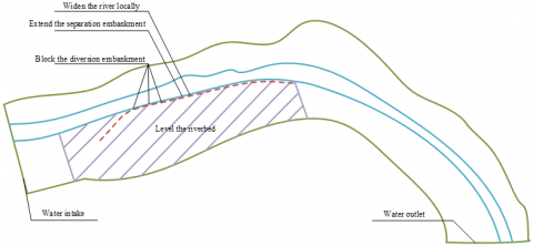
During the experiment of mathematical model and physical model, it is found that the existing navigation scheme of navigable tunnel cannot effectively improve the navigable flow conditions in the entrance area of the approach channel because of the uneven riverbed, sand dunes and deep grooves. In order to achieve ideal navigation conditions, it is necessary to widen the river locally, extend the separation embankment, block the diversion embankment, level the riverbed, or set up local dredging flood discharge channels and build water diversion structures. Schematic diagrams of different schemes are shown in Figure 1.
Figure 1. Schematic diagram of different schemes
Based on the medium water flow rate of 6000m3/s, the analysis and research on the flow conditions of small flow rate below this flow rate or large flow rate above this flow rate have certain reference. Due to the limitation of the study time, this article chooses several navigable tunnels under the conditions of 500m3/s, 1000m3/s, 2000m3/s, 4000m3/s, 6000m3/s, 8000m3/s, 1000m3/s, 12000m3/s for test. Table 1 gives the upstream and downstream water level difference of the physical model of navigable tunnel under different discharge levels.
Through adjusting roughness for many times and verifying calculation repeatedly, Table 2 gives the verification results of three level flows such as 2000m3/s, 6000m3/s and 12000m3/s. Through the comparison of water surface line between physical model and mathematical model, it can be found that the water level deviation of the two models is within 0.1 m, which meets the error requirements specified in the Technical Specification for Flow and Sediment Simulation of Inland Waterway and Port, and the consistency between water surface line and water surface gradient is high.
Figure 2 and Figure 3 show the verification results of water surface lines and water flow velocities of different sections of navigable tunnel. It can be seen from the figures that the constructed model is in good agreement with the actual situation of the surface flow velocity distribution in the sharp bay section, and the mainstream position and lateral change trend also maintain a good degree of coincidence. The surface velocity deviation of the two models is basically within ± 0.1m, and the maximum is less than 0.2m. It can be verified that the mathematical model and physical model constructed in this article meet the relevant requirements in geometric similarity, flow motion similarity and dynamic similarity.
Table 3 gives a summary of the maximum transverse velocity of each channel section within the entrance area of the approach channel under the physical model. The summary results shows, according to the preset research purpose and physical model experiment requirements, the area from the end of the navigation wall in the entrance area of the approach channel to 400m downstream is the action area of the anti-trajectory-bucket flow pier. In order to ensure that the end of the navigation wall is still affected and sheltered by the anti-trajectory-bucket flow pier, the anti-trajectory-bucket flow pier should be set within the transverse distance of less than 70m from the approach channel. Considering that the section from the end of the navigation wall to its downstream 150m is greatly affected by the discharge flow and the transverse distance between the anti-trajectory-bucket flow pier and the navigation wall, and the cross-flow intensity between the 150m ~ 200m section is the most prominent. Therefore, this article selects 150m section downstream of the end of the navigation wall to carry out the related research on ship navigation trajectory, rudder angle and drift angle.
Figure 4 shows the navigation test results of a ship with a section of 150m downstream of the end of the navigation wall and Figure 5 shows the navigation trajectory of the ship. It can be seen from the figures that when the average flow velocity of 150m section is 1.0m/s, the cross flow value of 2.5m of 10000t cargo ship with a length of 5m on the route exceeds the limit value. When the ship travels against the current and the speed is about 2.0m/s, the maximum drift angle is -10.54°, and the navigation parameters are not ideal. Only when the navigation speed is increased to over 3.0m/s, the navigation parameters can barely meet the requirements of the threshold value. When the ship travels downstream and the navigation speed is 1.5m/s and 2.0m/s, the maximum rudder angle reaches -22.30° and 21.64°, respectively, and the maximum drift angle reaches 9.67° and 9.96°, respectively. The navigation parameters are not ideal enough to ensure the safe passage of ships through the entrance area of the approach channel. Only when the navigation speed is increased to over 2.5m/s will the navigation parameters meet the requirements of the threshold value.
Table 1. Water level difference between upstream and downstream of navigable tunnel under different discharge levels
|
SN |
Corresponding flow |
Upstream reservoir water level |
Downstream water level |
Water level difference |
|
1 |
500 |
93.35 |
83.34 |
8.63 |
|
2 |
1000 |
94.17 |
84.72 |
7.82 |
|
3 |
2000 |
94.58 |
86.35 |
7.06 |
|
4 |
4000 |
96.41 |
87.52 |
7.74 |
|
5 |
6000 |
98.52 |
88.67 |
7.17 |
|
6 |
8000 |
99.27 |
89.35 |
7.86 |
|
7 |
10000 |
100.25 |
89.41 |
7.08 |
|
8 |
12000 |
100.41 |
90.57 |
5.88 |
Table 2. Comparison of water level calculated by mathematical model and physical model
|
Flow |
Water gauge No. |
Mileage |
Left bank |
Right bank |
||||
|
Mathematical model |
Physical model |
Deviation |
Mathematical model |
Physical model |
Deviation |
|||
|
2000 1000 500 |
1 |
-251 |
41.629 |
44.364 |
-0.058 |
43.629 |
43.629 |
0.093 |
|
2 |
569 |
49.581 |
48.572 |
-0.024 |
41.528 |
44.517 |
-0.041 |
|
|
3 |
1542 |
43.629 |
42.591 |
0.063 |
47.152 |
43.528 |
-0.027 |
|
|
4 |
3629 |
41.582 |
47.514 |
-0.058 |
46.295 |
48.251 |
-0.015 |
|
|
Tail water |
3471 |
40.639 |
43.625 |
0.041 |
43.152 |
47.625 |
0.016 |
|
|
6000 4000 2000 |
1 |
-258 |
46.152 |
46.298 |
0.029 |
48.327 |
41.025 |
-0.034 |
|
2 |
569 |
44.281 |
44.271 |
0.035 |
44.051 |
43.519 |
0.012 |
|
|
3 |
1152 |
47.629 |
43.581 |
0.041 |
43.629 |
47.642 |
-0.052 |
|
|
4 |
3514 |
43.522 |
46.295 |
-0.025 |
48.527 |
48.032 |
-0.069 |
|
|
Tail water |
3629 |
49.625 |
42.733 |
0.041 |
43.625 |
41.472 |
0.025 |
|
|
12000 10000 8000 |
1 |
-254 |
55.847 |
51.629 |
0.017 |
54.026 |
53.629 |
0.018 |
|
2 |
526 |
53.629 |
57.428 |
-0.069 |
53.629 |
57.418 |
0.052 |
|
|
3 |
1742 |
51.248 |
55.382 |
0.037 |
55.814 |
55.014 |
-0.041 |
|
|
4 |
3629 |
57.426 |
58.629 |
-0.024 |
57.324 |
53.629 |
-0.069 |
|
|
Tail water |
3274 |
53.629 |
56.412 |
0.025 |
51.247 |
57.441 |
0.035 |
|
Figure 2. Verification of water surface lines of different sections of navigable tunnel
Figure 3. Verification of flow velocity in different sections of navigable tunnel
Table 3. Maximum transverse velocity of navigable tunnel cross section under different schemes
|
Transverse distance Measured cross-sections |
No trajectory-bucket flow pier |
20m |
30m |
40m |
50m |
60m |
70m |
80m |
90m |
100m |
|
50m |
0.52 |
0.03 |
0.04 |
0.01 |
0.14 |
0.19 |
0.01 |
0.39 |
0.35 |
0.42 |
|
100m |
0.53 |
0.35 |
0.29 |
0.24 |
0.26 |
0.23 |
0.29 |
0.27 |
0.24 |
0.26 |
|
150m |
0.41 |
0.42 |
0.45 |
0.34 |
0.37 |
0.37 |
0.37 |
0.22 |
0.29 |
0.27 |
|
200m |
0.34 |
0.41 |
0.49 |
0.45 |
0.39 |
0.41 |
0.34 |
0.29 |
0.21 |
0.29 |
|
250m |
0.39 |
0.46 |
0.36 |
0.39 |
0.33 |
0.47 |
0.31 |
0.34 |
0.35 |
0.24 |
|
300m |
0.25 |
0.38 |
0.34 |
0.31 |
0.39 |
0.35 |
0.39 |
0.37 |
0.26 |
0.26 |
|
350m |
0.21 |
0.25 |
0.29 |
0.27 |
0.22 |
0.28 |
0.24 |
0.22 |
0.22 |
0.28 |
|
400m |
0.15 |
0.22 |
0.27 |
0.24 |
0.28 |
0.22 |
0.21 |
0.27 |
0.24 |
0.22 |
Figure 4. Rudder angle, drift angle and speed of ship navigation
Figure 5. Schematic diagram of ship navigation trajectory
When the average flow velocity of 150m section is 1.5m/s, the cross flow value of 2.75m of 10000t cargo ship with a length of 5m on the route exceeds the limit value. The maximum rudder angle is about 23.14° and the maximum drift angle is about -13.11° when the ship travels against the current and the speed is about 3.0m/s, so the navigation parameters are not ideal. Only when the navigation speed is increased to over 3.5m/s, the navigation parameters can barely meet the requirements of the threshold value. When the ship travels downstream at 2.0m/s and 2.5m/s, the maximum rudder angle reaches -22.45° and 21.73°, respectively, and the maximum drift angle reaches 11.23° and 11.92°, respectively. The navigation parameters are not ideal enough to ensure the safe passage of ships through the entrance area of the approach channel. Only when the navigation speed is increased to 3.0 ~ 3.5m/s will the navigation parameters meet the requirements of the threshold value.
This article studies the characteristics of navigation flow conditions and numerical simulation of water conservancy in steep bay section of the tunnel. Firstly, the physical model of tunnel navigation in steep bay section is designed to ensure the geometric similarity, flow movement similarity and dynamic similarity between the model and the actual situation in steep bay section. Then, the numerical simulation of navigation water conservancy in steep bay section of tunnel is carried out, and the continuity equation and momentum equation in the new coordinate system are given. This article explores the navigation scheme of large cross-section navigable tunnel in order to obtain effective measures to improve the navigation conditions of this section. Finally, by adjusting roughness several times and repeatedly validating calculation, this article obtains the validation results of three level flow rate such as 2000m3/s, 6000m3/s and 12000m3/s, which verifies the effectiveness of the physical model and mathematical model. It obtains the verification results of water surface lines and water flow velocities of different sections of navigable tunnels and further verifies that the mathematical model and physical model constructed have reached the relevant requirements in geometric similarity, flow motion similarity and dynamic similarity. It summarizes the maximum transverse velocity of each channel section in the entrance area of approach channel under the physical model, selects the section 150m downstream of the end of the navigation wall to study the ship's navigation trajectory, rudder angle and drift angle, and obtains the corresponding research results.
[1] Bazylev, A.V., Plyushchaev, V.I. (2021). Digital information system for inland water transport vessels based on AIS. In Journal of Physics: Conference Series, 2131(3): 032031. https://doi.org/10.1088/1742-6596/2131/3/032031
[2] Pantina, T., Borodulina, S. (2021). Assessment of regional transport accessibility indices for inland water transport services. In E3S Web of Conferences, 244: 11016. https://doi.org/10.1051/e3sconf/202124411016
[3] Piątek, D. (2019). New concept of hybrid propulsion with hydrostatic gear for inland water transport. Polish Maritime Research, 26(2): 134-141. https://doi.org/10.2478/pomr-2019-0033
[4] Pilechi, A., Mohammadian, A., Murphy, E. (2022). A numerical framework for modeling fate and transport of microplastics in inland and coastal waters. Marine Pollution Bulletin, 184: 114119. https://doi.org/10.1016/j.marpolbul.2022.114119
[5] Yan, M., Wang, L., Dai, Y., Sun, H., Liu, C. (2021). Behavior of microplastics in inland waters: Aggregation, settlement, and transport. Bulletin of Environmental Contamination and Toxicology, 107(4): 700-709. https://doi.org/10.1007/s00128-020-03087-2
[6] Scheepers, H., Wang, J., Gan, T.Y., Kuo, C.C. (2018). The impact of climate change on inland waterway transport: Effects of low water levels on the Mackenzie River. Journal of Hydrology, 566: 285-298. https://doi.org/10.1016/j.jhydrol.2018.08.059
[7] Łebkowski, A. (2018). Reduction of fuel consumption and pollution emissions in inland water transport by application of hybrid powertrain. Energies, 11(8): 1981. https://doi.org/10.3390/en11081981
[8] Voskresenskaya, E., Vorona-Slivinskaya, L., Ponomareva, T. (2018). Application of public-private partnership mechanisms for competitive growth of inland water transport in Russia. In MATEC Web of Conferences, 239: 08009. https://doi.org/10.1051/matecconf/201823908009
[9] Gao, S., Shi, S. (2021). Development suggestion of China inland water transportation in the new era situation. In Fifth International Conference on Traffic Engineering and Transportation System (ICTETS 2021), Vol. 12058, pp. 145-151. https://doi.org/10.1117/12.2619593
[10] Liu, Y., Jiao, J.J., Luo, X. (2016). Effects of inland water level oscillation on groundwater dynamics and land-sourced solute transport in a coastal aquifer. Coastal Engineering, 114: 347-360. https://doi.org/10.1016/j.coastaleng.2016.04.021
[11] Nowakowski, T., Kulczyk, J., Skupień, E., Tubis, A., Werbińska-Wojciechowska, S. (2015). Inland water transport development possibilities–case study of lower vistula river. Archives of Transport, 35(3): 53-62. https://doi.org/10.5604/08669546.1185192
[12] Kalina, T., Jurkovic, M., Grobarcikova, A. (2015). LNG-Great opportunity for the inland water transport. Transport Means, 22-23.
[13] Zhang, S.H., Wu, Y., Jing, Z., Yi, Y.J. (2018). Navigable flow condition simulation based on two-dimensional hydrodynamic parallel model. Journal of Hydrodynamics, 30(4): 632-641. https://doi.org/10.1007/s42241-018-0062-1
[14] He, C. (2020). Study on the impact of different pier structures on navigable flow conditions. In IOP Conference Series: Earth and Environmental Science, 560(1): 012061. https://doi.org/10.1088/1755-1315/560/1/012061
[15] Wen, C., Ran, G.J. (2012). Navigable flow condition numerical simulation for approach channel of tiangongtang junction. In Advanced Materials Research, 490: 2444-2448. https://doi.org/10.4028/www.scientific.net/AMR.490-495.2444
[16] Yang, Y., Shao, X., Qin, C., Zhou, J., Wang, Y. (2014). 3D numerical simulation of navigable flow conditions of river reach between Wudongde and Baihetan reservoirs. Tianjin Daxue Xuebao (Ziran Kexue yu Gongcheng Jishu Ban)/Journal of Tianjin University Science and Technology, 47(11): 994-1000. https://doi.org/10.11784/tdxbz201304051
[17] Zhang, S., Jing, Z., Li, W., Wang, L., Liu, D., Wang, T. (2019). Navigation risk assessment method based on flow conditions: A case study of the river reach between the Three Gorges Dam and the Gezhouba Dam. Ocean Engineering, 175: 71-79. https://doi.org/10.1016/j.oceaneng.2019.02.016
[18] Aminzadeh, A., Atashgah, M.A. (2018). Implementation and performance evaluation of optical flow navigation system under specific conditions for a flying robot. IEEE Aerospace and Electronic Systems Magazine, 33(11): 20-28. https://doi.org/10.1109/MAES.2018.170075
[19] Ma, D.G., Liu, X., Zhao, J.Q., Liu, X.F., Li, S.X. (2011). The research of navigation flow conditions and improvement measures on entrance area and connecting reach of Dahua Lock in Hongshui River. In Advanced Materials Research, 250: 3624-3629.
[20] Yao, S.M., Wang, X.K., Zhang, C., Zhang, D.W. (2007). 3-D numerical simulation of navigable flow conditions between Three Gorges Dam and Gezhouba Dam. Advances in Water Science, 18(3): 374-378.
[21] Liu, Y., Li, X. (2006). Study on the navigation flow condition at entrance area of the ship approach channel for Jinghong power station on the Lancang river. Journal-Chongqing Jianzhu University, 28(5): 55-58+62.
[22] Deng, B., Wang, M.F., Jiang, C.B., Wu, Z.Y. (2021). Propagation characteristics of ship waves in navigation tunnel and its influence on continuous navigation safety of ship. Kexue Tongbao/Chinese Science Bulletin, 66(9): 1101-1112. https://doi.org/10.1360/TB-2020-0124
[23] Yang, Y., Zhang, Z., Cheng, W., Wang, R. (2021). Analysis of navigation flow conditions in the entrance area of the Babao ship lock of Hangzhou section of Jinghang Grand Canal. In IOP Conference Series: Earth and Environmental Science, 643(1): 012140. https://doi.org/10.1088/1755-1315/643/1/012140
[24] Böttner, C.U., Anschau, P., Shevchuk, I. (2020). Analysis of the flow conditions between the bottoms of the ship and of the waterway. Ocean Engineering, 199: 107012. https://doi.org/10.1016/j.oceaneng.2020.107012
[25] Wu, T., Ding, J. (2013). Experimental study on flow conditions of Jiaogang ship lock during sluice gate hoist. Applied Mechanics and Materials, 405: 1458-1462. https://doi.org/10.4028/www.scientific.net/AMM.405-408.1458