Joseph Magdi* | Irene Samy | Ehab Mina
© 2022 IIETA. This article is published by IIETA and is licensed under the CC BY 4.0 license (http://creativecommons.org/licenses/by/4.0/).
OPEN ACCESS
A new photovoltaic technology is manufactured from an organic material that easily degrades in nature. Unfortunately, organic photovoltaics suffer from low thermal stability and lower power conversion efficiency compared with silicon-based photovoltaics. Cooling is critical in this type of photovoltaic because of these factors. This research investigates a new method to cool this organic photovoltaic with a heat pipe to achieve a minimum operating temperature and maximum temperature uniformity, the heat pipe design is fixed, and the number of cells served by a single heat pipe is studied. For each case, the temperature distribution is plotted, and the maximum and the range in the temperature distribution are recorded, respectively, as a measure of the cell's performance. The temperature of the cell is evaluated numerically using COMSOL 5.6 Multiphysics™ software with and without the heat pipe. The electrical performance was estimated in both cases using GPVDM™ software. Consequently, the combined system of panel and cell reaches a maximum thermal stability at a minimum temperature of 33.4℃ instead of 52℃ without a heat pipe, which improves the electrical performance and the power conversion efficiency by 0.24%.
heat transfer, renewable energy, organic photovoltaic, heat pipe, thermal stability
Advances in renewable energy technologies is a key factor toward achieving a smart and sustainable future. Organic photovoltaics is a promising technology that is anticipated to be a significant source of energy production due to its advantages over silicon-based solar cells, including low production costs and large-area manufacturing processes using conventional industrial roll-to-roll techniques like coating and printing [1]. This research will investigate the enhancement in efficiency and stability of organic solar cells. However, the most popular and widely used active layer material (P3HT: PCBM) can be used by coupling that cell with a copper-based heat pipe, one of the appealing alternatives that increase the usage of renewable energy is PV technology, which has the ability to meet around 5% of the world's electricity consumption by 2030 and 11% by 2050 [2]. Despite the PV technology's immense potential, several problems, like as low conversion efficiency, high temperatures, and dust collection, have made it difficult to use widely [3].
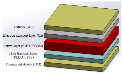
The organic photovoltaic panels have a great advantage to environment because they are made from biodegradable materials. Unfortunately, Organic Photovoltaics (OPV) have a much lower efficiency compared to silicon base cells. This opens up the possibility of looking into the development of recyclable (polymer) solar cells, which is one of the main the subject s of this study. OPV devices are comprised of a number of layers. In the standard configuration as shown in Figure 1.
A transparent conductor that acts as the anode is deposited on a transparent substrate (glass or plastic). A hole-transport buffer layer that sits between the anode and the absorbing active layer keeps electrons from getting to the anode. A similar electron-transport buffer layer serves the analogous function on the opposite side of the active layer, followed by the (optically reflecting) cathode.
Figure 1. Schematics of common layer structure of OPV devices in normal geometry with typical materials noted
The relatively low stability of organic photovoltaic materials is one of the key obstacles impeding their widespread manufacture. Stability requirements depend exclusively on the application where the OPV will be used. However, If the resulting gadget lifespan is inadequate for the technical needs, achieving high performance has minimal technological benefit. According to consensus stability testing methodologies for organic photovoltaic materials and devices, the applied temperatures as high as 65-85℃ are a critical factor that has to be regulated for outdoor applications [4]. But in actual condition the top surface of OPV cell reach 51.8℃ [5].
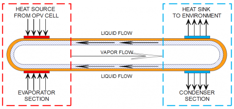
Heat pipes are two-phase flow elements with excellent thermal conductivity that allow liquid to go from the condenser to the evaporator and inversely [6]. Using a condensable fluid contained in a sealed chamber, heat is transmitted from the heat source (the evaporator portion of the heat pipe) to the heat sink (the condenser section of the heat pipe). In essence, the heat source's absorption of heat in the evaporator zone causes the liquid to evaporate. As the vapor enters the condenser section, it condenses and releases its latent heat. By use of capillary force, the liquid is returned to the evaporator region and re-vaporized there to complete the process [7]. The temperature differential over the whole length of the pipe is reduced because the vapor pressure loss is intended to be nearly zero as the vapor moves from the evaporator region to the condenser section [6]. Because of this, both sections have equal saturation temperatures (temperatures at which evaporation and condensation occur), Also the different in temperatures leads to different density respectively which will produce a convectional heat as illustrated in Figure 2.
Figure 2. Components and principle of operation of a conventional heat pipe
The increase of OPV cell temperature under the normal incident radiation of sunlight affects the general behavior of the cell performance by decreasing the open-circuit voltage which causes the power output to drop [8]. This drop will be shown in details at the result and discussion section. While at this current state of research the efficiency of PV panels is impacted by the fact that a conventional cooling cycle using air or water is unable to maintain a uniform temperature distribution all throughout the panel [9]. Another solution was established by Zainal Arifin and et al. that enhances PCE of the PV panels by 0.42% using a Soybean Wax as a phase change material for cooling [10]. However, heat pipes offer a solution to this problem through an enhancement in heat transfer rate.
This paper compares the performance of a PV panel that is cooled by heat pipe. The heat pipe design is fixed and the number of cells served by a single HP is studied. For each case, the temperature distribution is plotted and the maximum and the range in temperature distribution are recorded respectively, as a measure of the cell performance.
Model for General-Purpose Photovoltaic Device (GPVDM). The starting condition efficiency of light harvesting systems may be calculated using the free general-purpose tool GPVDM. In the program handbook, the model is described in greater detail [10]. The software gives an output that contains the Current-Voltage (I-V) characteristic curves [11].
A useful tool that may be used in many different engineering domains is Comsol Multiphysics. The physical governing equations have been solved using the finite element technique (FEM) by this program. The goal of the current study is to give an extensive evaluation of the numerical research conducted using Comsol Multiphysics due to the significance of heat transfer in modern heat pipe technologies and the potential of numerical approaches in the resolution of related problems.
2.1 Problem discerption
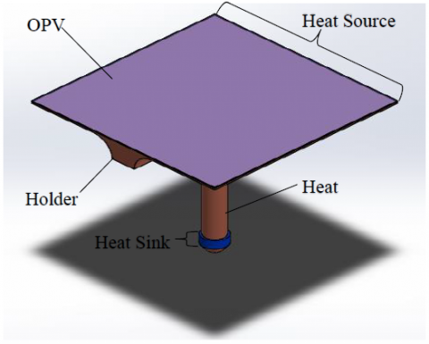
The combined OPV-HP system works rather simply by impinging solar radiation onto the PV surface, which causes the cell to heat up and increase in temperature as a result of the radiation and the surrounding environment. Following the transmission of the radiation into each PV layer, some of it is directly [12] transformed into electricity by the active layer, while the remainder is lost to the environment due to radiation and convection. Conduction is used to transport the leftover heat to the associated HP module, supplying the input heat flux required by the HP. In the case of the OPV-HP, the condenser is located on the free end surface, and the PV is affixed to the top surface of the heat pipe (HP) evaporator. Solar radiation impinges on the upper surface of the PV modules that are mounted to the flat plate evaporator when the hybrid system is in operation. The working fluid in liquid form is vaporized by the heat input at the wick surface in the evaporator section, and the vapor and its latent heat subsequently move in the direction of the cooler condenser section. Heat is released from the heat pipe working fluid in the condenser section, and this heat is returned to the evaporation section through conduction and the gravitational surface tension action of the inner liquid. Subsequently, then that process will be repeated continuously to achieve the thermal equilibrium and maintain high thermal stability of the system as shown in Figure 3.
Figure 3. Theory of operation and schematic view of the combined models (OPV cell, Model holder, and Heat pipe)
2.2 Material properties
For the GPVDM OPV model simulator software this research paper has used the most common active layer material of organic photovoltaics type P3HT:PCBM [13] and Table 1 shows the parameters used in the simulation.
Table 1. General parameters of OPV cell design
|
Parameter |
Value |
|
Electron trap density |
3.8000e26 $m^{-3} \mathrm{eV}^{-1}$ |
|
Hole trap density |
1.4500e25 $m^{-3} \mathrm{eV}^{-1}$ |
|
Electron tail slope |
0.04 $\mathrm{eV}$ |
|
Hole tail slope |
0.06 $\mathrm{eV}$ |
|
Electron mobility |
2.48e-07 $m^2 V^{-1} S^{-1}$ |
|
Hole mobility |
2.48e-07 $m^2 V^{-1} S^{-1}$ |
|
Relative permittivity |
3.8 $a u$ |
|
Number of traps |
20 bands |
|
Free electron to Trapped electron |
2.5000e-20 $m^{-2}$ |
|
Trapped electron to Free hole |
1.3200e-22 $m^{-2}$ |
|
Trapped hole to Free electron |
4.6700e-26 $m^{-2}$ |
|
Free hole to Trapped hole |
4.8600e-22 $m^{-2}$ |
|
Effective density of free electron states |
1.2800e27 $m^{-3}$ |
|
Effective density of free hole states |
2.8600e25 $m^{-3}$ |
|
Bandgap |
1.1 $\mathrm{eV}$ |
The optical properties of the OPV cell used in this study were performed through GPVDM software parameters, therefore the active layer material thickness applied for this analysis is adjusted to be 220 nm as the most effective thickness performance which has the lowest recombination rate and the maximum efficiency [13]. However, for COMSOL Multiphysics™ software used copper as heat pipe material for the best thermal conductivity and water as working fluid which is described briefly later on section.
In this research the numerical analysis will divided into three sections to simplify the modeling and due to the different software used for each section as following:
3.1 Photovoltaic model
By examining its current-voltage characteristics curve, it is possible to determine the major electrical features of a solar panel. When the voltage is equal to zero, the current is said to be in a short circuit, and when the voltage is equal to zero, the current is said to be in an open circuit. the voltage at the maximum power point and the maximum power point When the power output is at its highest, the voltage and current are, respectively, the voltage and current. The point when the product of the current and voltage is at its highest value is known as the maximum power point. The fill factor is the ratio of the maximum power point by a solar cell and the product of Voc and Jsc. Empirically the FF is given by [8]:
$F F=\frac{v_{o c}-\ln \left(v_{o c}+0.72\right)}{v_{o c}+1}$ (1)
$v_{o c}=\frac{q}{n k T} V_{o c}$ (2)
The ratio of the maximum produced power to the incident power is used to calculate conversion efficiency. Test conditions are used to measure solar cells (STC), where the incident light is described by the AM1.5 spectrum and has an irradiance of 1000 W/m2 [14].
The governing equations, for the temperature distribution in each layer of the PV are given as [15]:
$\rho C_P \frac{\partial T}{\partial t}-\nabla \cdot(K \nabla T)=\dot{q}_{\text {sol }}-\dot{P}_{g e n}$ (3)
The electrical power generation per volume which is zero for all layers except the active material cell layer.
By initially defining the solar radiation intensity, the solar energy absorption and power generation in each layer of the PV can be modeled. The energy absorption in each layer can then be estimated and taken into account as an internal heat generation. In this investigation, it is assumed that the cell surface is constantly lit evenly. The volumetric energy absorption of each layer is given as:
$\dot{\mathrm{q}}_{\mathrm{sol}, \mathrm{i}}=\frac{\mathrm{G}_{\mathrm{rec}, \mathrm{i}} \times \alpha_{\mathrm{i}} \times \mathrm{A}_{\mathrm{i}} \times \mathrm{C}}{\mathrm{V}_{\mathrm{i}}}$ (4)
$\mathrm{G}_{\mathrm{rec}, \mathrm{i}}=\mathrm{G}_{\text {rec }, \mathrm{i}-1}\left[\left(1-\alpha_{i-1}\right)-\rho_{i-1}\right]$ (5)
In the active layer of OPV cell, Pgen power generation is considered as an internal heat sink and can be defined as [16]:
$\eta_{p v}=\eta_{r e f}\left[1-\beta\left(T_{c e l l}-T_{r e f}\right)\right]$ (6)
The sky temperature used for the radiative heat loss calculation at the surface of the PV is given as [17]:
$T_{s k y}=0.0552 \times T_a^{1.5}$ (7)
The convective heat transfer coefficient of air is obtained by free natural convection around the cell because the average air velocity in Cairo is about 3.78 m/s [18], thus start with the simple empirical correlations for the average Nu in natural convection are of the form [19]:
$N u=\frac{h L_c}{k}=C\left(G r_L \operatorname{Pr}\right)^n=C\left(R a_L\right)^n$ (8)
where, C and n are a constants depending on the geometry of the surface and the flow regime, which is characterized by the range of the Rayleigh number.
$R a_L=G r_L \operatorname{Pr}=\frac{g \beta\left(T_S-T_{\infty}\right) L_c^3}{v^2} \operatorname{Pr}=\frac{g \beta\left(T_s-T_{\infty}\right) L_c^3}{v \alpha}$ (9)
So after calculated Rayleigh number with air properties at 38.4℃ film temperature, the constants of C and n can be found by solving the Nusselt Number [20]:
$N u=0.1(R a_L)^{\frac{1}{3}}$ (10)
Then the convective heat transfer coefficient of air can be found at the top and the bottom of cell surface.
The characteristics length is established using the following formula:
$L_{c h}=\frac{\mathrm{A}_{\mathrm{sur}}}{p}$ (11)
Theses dimensionless parameters calculated and used their values as an input parameter to the hybrid model.
Boundary conditions for accurate the PV model, the following boundary conditions are applied, and some assumptions are considered to simplify the model with minimal deviation from the real case.
3.2 Heat pipe model
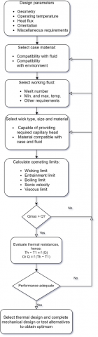
A simplified heat pipe model is used in this research and modified to achieve the OPV cooling requirements which in this case the most parameter is absorbing some heat flux from the outer surface of the cell to make it more efficient and reliable, the flow chart design concept sequence of heat pipe is showing in Figure 4.
Material choices for the container: The container's function is to keep the working fluid isolated from the environment. It must thus be impervious to leaks, keep a differential pressure across its walls, and permit heat transfer into and out of the working fluid. The following are some of the numerous aspects that influence the material choice for containers:
In this research the container material is copper which has the finest thermal conductivity than other materials such as aluminum or steel, and also compatible with the working fluid and the wick material and has archive most of factors that was mentioned before.
The selection of an acceptable working fluid is the most crucial aspect of the design and development processes. Operating temperature, latent heat of vaporisation, liquid viscosity, toxicity, chemical compatibility with container material, wicking system design, and performance requirements are only a few of the factors that affect the choice of working fluid. The normal operating temperature range of a heat pipe is between its critical temperature and the triple state of the working fluid. However, for most heat pipe applications for electronic thermal control, the working fluid must be chosen to have a boiling point between 250 and 375 K [23]. The effectiveness of various working fluids at particular operating temperatures can be evaluated using the liquid transport factor, also known as the figure of merit. Due to its high latent heat of vaporization, acceptable viscosity, cheap cost, and high "figure of merit," water is selected as the working fluid for this study [24].
Figure 4. Heat pipe design sequence
Wick structural selection: A wick's main job is to provide capillary pressure to transfer the working fluid from the condenser to the evaporator; as pore size decreases, a wick's maximal capillary pressure differential rises. The wick's permeability decreases with smaller pores, and increasing wick thickness causes a reduction in the vapor core volume [25]. There are several wick structural varieties, but the most popular is the homogeneous type, which is implemented in this work as a sintered homogenous wick that increases the capillary effect to improve the operation.
3.2.1 The operational limits
Are affected by the working fluid, wick characteristics, pipe size and shape, operating temperature, and heat transfer constraints. The maximum heat transfer limitation of a heat pipe at a specific temperature is determined by the lowest limit among these constraints [6]. These limits are the most important part of heat pipe design which is to restrict and calculate how efficient this design is. This research will make wide explanations for each limit as following:
Wicking/Capillary or Circulation Limit. In the event that the heat pipe is in a steady state of operation, there is a constant flow of liquid via the wick from the condenser section to the evaporator section and vapor from the evaporator section to the condenser section. The maximum heat flux allowed can be calculated by balancing the internal pressures in all heat pipe sections (condenser, adiabatic, and evaporator). The vapor pressure gradient ($\Delta p_v$) and the liquid pressure gradient ($\Delta p_l$) throughout the length of the heat pipe makes these flows conceivable. Additionally, due to the inclination, the gravity pressure ($\Delta p_g$) to be taken, allowing the capillary pressure to be represented as:
$\Delta P_{\text {capillary }, \text { max }}=\Delta P_l+\Delta P_v+\Delta P_g$ (12)
where the maximum capillary pressure for cylindrical pores can be calculated by:
$\Delta P_{\text {capillary }}=\frac{2 \sigma_l}{r_{e f f}}$ (13)
where, reffis the effective capillary radius or pores of the wick in and σl is the liquid surface tension. For a steady-state mode (constant heat addition and removal) and little manipulation and integration over the length of heat pipe the liquid pressure gradient can be written as:
$\Delta P_l=\frac{\mu_l \dot{Q} l_{e f f}}{\rho_l L A_w k}$ (14)
where, µl the liquid viscosity, ρl is the liquid density, leff is effective heat pipe length, Aw is the wick cross-sectional area, L is the latent heat of vaporization and K is permeability represents a property of the wick structure. Also for simplicity of analysis the vapor pressure gradient in neglected due to the low value compared with liquid pressure gradient. However, the wick permeability can be find as following:
$K=\frac{2 \varepsilon r_{l l}^2}{\left(f_l \operatorname{Re}_l\right)}$ (15)
where, Rel is the Reynold’s number of liquid, fl is the friction factor, ε is the wick porosity which is used equal to 0.5 as volumetric void fraction in wick and K is taken as 1E-9 m2. Thus the heat transport factor $(Q L)_{\text {capillary } \max }$ is calculated by:
$(\mathrm{QL})_{\text {capillary }_{\max }}=\frac{\frac{2 \sigma}{\mathrm{r}_{\mathrm{c}}}-\Delta P_{\perp}-\rho_l g L_{\text {total }} \operatorname{Sin} \psi}{F_l+F_v}$ (16)
where, rc is the effective capillary radius, $\Delta P_{\perp}$ is hydrostatic pressure in direction perpendicular to pipe axis, ψ is heat pipe inclination measured from horizontal position and Fl, Fv is frictional coefficient for liquid flow and frictional coefficient for vapor flow respectively. These coefficients are expressed as:
$F_l=\frac{\mu_l}{K A_w{ }^h f_g \rho_l}$ (17)
$F_v=\frac{\left(f_v \operatorname{Re}_v\right) \mu_v}{2 r_{h_v}^2 A_v \rho_v h_{f g}}$ (18)
And finally maximum capillary or wicking limitation for a conventional heat pipe operating under normal heat pipe mode is given by:
$Q_{\text {capillary }_{\max }}=\frac{(\mathrm{QL})_{\text {capillary }_{\max }}}{\left(0.5 L_c+L_a+0.5 L_e\right)}$ (19)
where, Le is the evaporator length, Lc is the condenser length and La is the adiabatic length.
Entrainment limit. A shearing force is applied to the liquid at the liquid-vapor contact as the liquid and vapor travel in opposite directions. If this shear force is greater than the liquid's surface tension, liquid droplets are entrained into the vapor flow and delivered to the condenser region. If this shear force is too great, it can dry up the evaporator since it depends on the vapor's velocity and thermophysical characteristics [26]. Maximum entrainment in high vapor velocities, the wick's liquid droplets are torn away from it and thrown into the vapor, which causes dryout. Only a composite or two-layer wick can be considered for the entrainment limit when the liquid recession is limited to the capillary pumping layer and the flow channel layer remains full [6]. Therefore, in this case the heat pipe model has single wick layer thus this limit can be neglected.
Boiling limit. When the input flux is enough, nucleation sites develop inside the wick and trapped bubbles prevent liquid from returning, leading to evaporator dryout. All other limitations are caused by insufficient axial heat flux, whereas the boiling limit is caused by excessive radial heat flux. The maximum heat flow over which bubble development and subsequent dryout will occur is given by [26]:
$\mathrm{Q}_{\mathrm{b}_{\max }}=\frac{2 \pi \mathrm{L}_{\mathrm{e}} \mathrm{k}_{\mathrm{e}} \mathrm{T}_{\mathrm{v}}}{\mathrm{h}_{\mathrm{fg}} \mathrm{r}_{\mathrm{v}} \ln \left(\mathrm{r}_{\mathrm{i}} / \mathrm{r}_{\mathrm{v}}\right)}\left(\frac{2 \sigma}{\mathrm{r}_{\mathrm{n}}}-\mathrm{P}_{\mathrm{c}}\right)$ (20)
where, Ke is the effective thermal conductivity of the liquid-saturated wick.
Sonic velocity limit. When the velocity of the vapor leaving the evaporator at a sonic speed. The vapor flow is “choked” and the maximum heat transfer rate is therefore limited. When the Mach number at the evaporator exit is equal, the unity and then the vapor velocity reaches the sonic limit and the sonic limitation at evaporator takes place. In this case, the sonic limit will be represented by:
$\mathrm{Q}_{\mathrm{S}_{\max }}=\mathrm{A}_{\mathrm{v}} \mathrm{r}_{\mathrm{v}} \mathrm{h}_{\mathrm{fg}}\left[\frac{\mathrm{g}_{\mathrm{V}} \mathrm{R}_{\mathrm{v}} \mathrm{T}_{\mathrm{v}}}{2\left(\mathrm{~g}_{\mathrm{v}}+1\right)}\right]^{1 / 2}$ (21)
Viscous limit. The development of the vapor-pressure restriction (or viscous limitation) in heat pipes occurs when the pressure drop in the vapour core is equal to the volume of the vapour in the evaporator. Due to the pressure drop caused by the flow through the vapour core under these circumstances, the condenser's vapour pressure is so low that the vapour cannot flow there.
$\mathrm{Q}_{\text {vapor } \text { max }_{\max }}=\frac{A_v r_v^2 h_{f g} \rho_{v_e} P_{v_e}}{16 \mu_{v_e} L_{\text {eff }}}$ (22)
3.2.2 Boundary conditions
To accurate the plate heat pipe model, the following boundary conditions are applied, and some assumptions are considered to simplify the model [26, 27].
Porosity ¢=0.5 is used with The Sintered copper powder wick.
3.2.3 Design parameters
The heat pipe COMSOL model configuration design criteria are setup for the most effectiveness parameters as shown in Table 2.
3.3 Hybrid model (Combine)
In this work, passive cooling via a heat pipe device with no electrical contribution to the hybrid system is considered, and the models of the PV and Heat pipe are integrated in terms of a Hybrid Thermal Model. Meanwhile, the heat pipe cools the PV, increasing its efficiency over time.
3.4 Computational domain
Software called COMSOL 5.6 Multiphysics™ is used to carry out the finite element-based numerical simulations in three dimensions for this investigation. The numerical investigation is conducted using the heat transfers in the medium of solid and liquid, the laminar flow interface, and the electric current interface. Boundary heat flux is utilized to take heat transfer in the liquid for the vapor chamber into consideration in order to appropriately quantify the convective heat flux. The terms “domain heat source” and “surface-to-ambient radiation interface” are used to describe the energy absorption in each PV layer and radiative heat loss, respectively. Additionally, a porous media interface is provided to the wick, and a heat sink boundary condition is applied to the heat pie’s cold side. The laminar flow interface is set up with a normal flow direction and an inlet boundary condition with saturation pressure at the top surface of the vapour chamber. A no-slip wall condition is also utilized. The solar radiation intensity (G0) is 1000W/m2 in all simulations, however variable concentration ratios are used to enhance this intensity. The numerical research is also performed out using a fully coupled direct linear solver in addition to the built-in COMSOL PARDISO (Parallel Sparse Direct Solver).
Table 2. Design parameters of heat-pipe design
|
Name |
Expression |
Description |
|
$r_{\text {outer }}$ |
10 [mm] |
Outer radius of pipe |
|
$w_{\text {casing }}$ |
1 [mm] |
Casing thickness |
|
$w_{\text {wick }}$ |
3 [mm] |
Wick thickness |
|
length |
150 [mm] |
Pipe length |
|
wick $_{\text {porosity }}$ |
0.5 |
Volumetric void fraction in wick |
|
wick $_{\text {permeabi }}$ |
1E-9 m² |
Permeability of wick |
|
$l_{\text {heatsink }}$ |
10 [mm] |
length of heat sink after rounded cap |
|
$l_{\text {heatsource }}$ |
10 [mm] |
length of heat source after rounded cap |
|
$w_{\text {contact }}$ |
10 [mm] |
Contact Surface Thickness |
|
Toperation |
- |
Operation Temperature |
|
$Q_{\text {in }}$ |
30 [W] |
Heat Source Load (Absorbed form Holder) |
|
$p h i_{\text {in }}$ |
Q_in/2/pi/r_outer/(r_outer+l_heatsource) 23873 [W/m²] |
Heat flux in (Absorbed form Holder) |
|
$O$ |
Vertical |
Orientation |
|
$p_{\text {ref }}$ |
1000 [Pa] |
Reference Pressure |
|
$h_{\text {conv }}$ |
1200 [W/(m²·K)] |
Convection coefficient heatsink |
3.5 Model validation
There are many different methods of validation established and divided into two sections as follows:
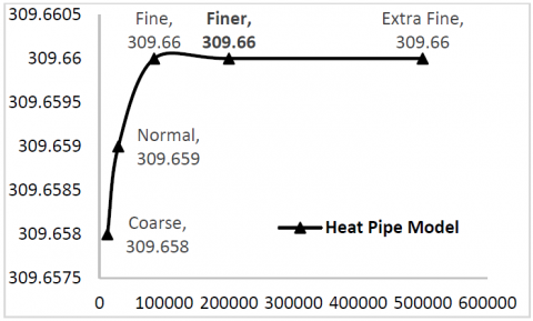
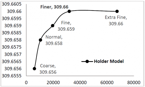
Firstly, in order to configure adequate independence of the mesh size and grid independency convergence for the heat pipe model in COMSOL software, the average temperature and the grid mesh with various element sizes was utilized as indicated in Figure 5. Same as the hybrid PV-HP system as indicated in Figure 6. It is evident that using the Finer mesh causes the average cell temperature and total hybrid system power output to converge. Therefore, the Finer Mesh is employed in all of the simulations for better accuracy and to save computing time.
Secondly, to validate the model and numerical simulation approaches utilised in this study, a comparison is made with experimental investigation and older studies that may be found in the literature. The HP simulation seen in the study of Zohuri [6] is used to confirm the current HP model utilised in these numerical simulations, and the identical circumstances employed in this work are set for accurate comparison. The PV simulation seen in the study of Shittu et al. [28] is used to validate the present PV model in this study. Simulation conditions are reset to those presented by Shittu et al. [28].
Figure 5. The average temperature with the grid independence of element sizes for heat pipe model
Figure 6. The average temperature with the grid independence of element sizes for cell holder model
The heat pipe model applied in this research is the same model that COMSOL Multiphysics™ offers in their application gallery [29]. There is no need to validate this model as a result. The geometrical proportions have, however, been altered for the purposes of the current study, which is important to note.
This study aims to present an applicable solution to generally enhance the electrical output from an OPV module cell through a novel idea, which is cooling by a heat pipe. Recently, this cooling technology has been used to enhance the conversion efficiency of the silicon-based photovoltaic-thermoelectric system [25]. However, A comparative result of a several numbers of cells and different geometrical dimensions was not done completed. This study investigates the relative size of OPV and HP to obtain adequate cooling for optimum operation. It is a novel optimum design that is modelled into two Comsol models, and their results are taken for the GPVDM OPV model as an input parameter to maintain the exact conversion efficiency for each case, where the simulation results can be divided into three sections as follows.
4.1 The thermal temperature distribution simulation of module holder model
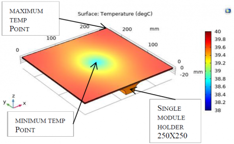
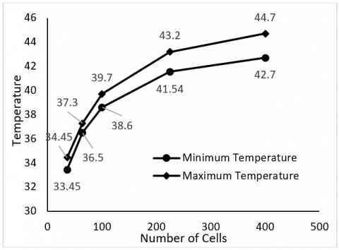
The first a module copper holder contains 100 cells with dimensions of 250X250X1 mm length, width, and thickness shown in Figure 7. which achieves thermal balance at temperature of 38.61℃. The second module holder contains 64 cells with dimensions of 200X200X1 mm length, width, and thickness achieves thermal balance at temperature of 36.5℃. And lastly the third module holder contains 36 cells with dimensions of 150X150X1 mm length, width, and thickness which achieves a thermal balance at temperature of 33.44℃. The model starting from the maximum initial temperature at 51.8℃ ending with the final heat balancing temperature.
Figure 7. Temperature distribution for a 100 cell module holder with dimensions of 250X250X1 mm – 3D upside view
A thermal contour diagram is presented in Figure 8, which details each location and its calculated temperature in degrees Celsius. This is performed in order to fully understand the thermal behavior and temperature distribution of the OPV-HP model. It is significant to mention that the farthest point from the cooling heat pipe at the center of the holder module contains the highest temperature. On the other hand, the closest point to the cooling surface of the heat pipe, where the middle of the holder module is the coldest point.
Figure 8. Temperature distribution contours for a 100 cell module holder – 3D upside view
4.2 The thermal temperature distribution simulation of heat pipe model
The maximum temperature point is at the interface between the heat pipe model and the cell holder model (considered as a heat source of the heat pipe model) and assumes a constant amount of absorption heat per the same heat pipe specifications. The combination model of OPV-HP will maintain a thermal equilibrium distribution at a certain temperature, therefore the more cells sets on one single holder mean more surface area and more heat required to absorb from that surface holder to maintain the same equilibrium temperature. The first heat pipe simulation model achieves thermal balance temperature with the module holder at 38.61℃ which generates an abstraction of heat from the cells by 19.603 W as shown in Figure 9. The second heat pipe simulation model achieves thermal balance temperature with the module holder at 36.5℃ which generating an abstraction of heat from the cells by 16.567 W. And the third heat pipe simulation model achieves thermal balance temperature with the module holder at 33.44℃ which generating an abstraction of heat from the cells by 12.162 W.
Figure 9. Temperature distribution for a heat pipe model working with a 100 cell module holder – 3D view
The established equilibrium temperature is affected by the varying cells number; conversely, as more cells are combined into one heat pipe, a higher temperature is attained. As a result, it can be deduced that adding additional cells to a heat pipe results cheaper initial cost but a lower effective efficiency. Furthermore, fewer cells with the same heat pipe characteristics will cost more while also being more efficient. This makes the cell number on a single heat pipe, as shown in Figure 10, a crucial design element for optimization.
Figure 10. The influence of cell number on one single heat pipe as result of COMSOL model
4.3 OPV cell simulation
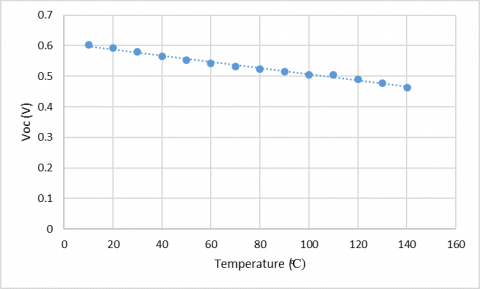
The following Figure 11 illustrates the relationship between open circuit voltage and temperature variation as a result of the GPVDM software cell model. As stated in the introduction section, the cell temperature remains constant at a low temperature throughout the entire day with heat pipe than equivalent cell without, therefore efficiency will increase as result of the temperature stability.
Figure 11. The Calculated and experimental values of open-circuit voltage as a function of temperature
The cell now maintains thermal stability at the same temperature as the module holder thus each combined holder-heat pipe model will make the cell generate a new power conversion efficiency as shown in Figure 12.
Figure 12. The influence of Heat pipe cooling technology on the cell efficiency
One of the biggest difficulties in OPV technology is the optimization of organic solar cells. In order to clarify and comprehend solar cell performance, a number of sophisticated mathematical methods were devised. In this research, the main objective is to enhance the temperature distribution of the polymer organic solar cell consequently its performance throughout a novel idea that combining a heat pipe cooling device which control the thermal behavior and distribution of the temperature across all the OPV cell then as a result the power conversion efficiency is stabilized under the daylight hours. The numerical model for each of OPV cell, HP and the combination was illustrated the point of this work associated with several validations. It was found that the Heat pipe device and technology to be very useful in precisely optimizing solar device performance, and improve their efficiency by 0.24%.
Maybe the impact of the cooling technology by Heat pipe on this type of solar cell is not much as other types of cell material like silicon solar cell or even the perovskite material that combines the organic polymer of OPV cell with silicon type which leads to enhance their physical properties when using this cooling technology of heat pipe.
|
OPV |
Organic Photovoltaics |
|
I-V |
Current-Voltage |
|
HP |
heat pipe |
|
Isc |
short circuit current |
|
Voc |
open- circuit voltage |
|
Vmpp |
maximum power point voltage |
|
Impp |
maximum power point current |
|
MPP |
maximum power point |
|
FF |
fill factor |
|
η |
power conversion efficiency |
|
voc |
normalized Voc |
|
ρ |
density |
|
Cp |
specific heat capacity |
|
k |
thermal conductivity |
|
T |
temperature |
|
qsol |
volumetric solar energy absorption by each layer |
|
$\dot{P}_{\text {gen }}$ |
electrical power generation per volume |
|
αi |
absorptivity |
|
ρi |
reflectivity |
|
Vi |
volume |
|
Grec,i |
the solar radiation intensity in each layer |
|
$\dot{q}_{s o l, i}$ |
the associated volumetric heat capacity at each layer |
|
Ai |
the area of each layer |
|
$C_{\text {solar }}$ |
the solar concentration ratio |
|
Pgen |
power generation |
|
ηref |
reference efficiency |
|
Tref |
reference temperature |
|
Tcell |
cell temperature |
|
$\beta_{\text {cell }}$ |
temperature coefficient |
|
Tsky |
sky temperature |
|
Ta |
ambient temperature |
|
h |
convective heat transfer coefficient |
|
k |
thermal conductivity of air |
|
Lc |
characteristic length |
|
GrL |
Grashof number |
|
Pr |
Prandtl number |
|
RaL |
Rayleigh number |
|
C |
constants depending on the geometry of the surface |
|
n |
constants depending on the flow regime |
|
β |
coefficient of volume expansion |
|
Tf |
film temperature |
|
Ts |
surface temperature |
|
T∞ |
ambient temperature |
|
g |
gravitational acceleration |
|
v |
kinematic viscosity |
|
α |
thermal diffusivity |
[1] Chidichimo, G., Filippelli, L. (2010). Organic solar cells: Problems and perspectives. Int. J. Photoenergy, 2010: 123534. https://doi.org/10.1155/2010/123534
[2] Diallo, T.M.O., Yu, M., Zhou, J., Zhao, X., Shittu, S., Li, G., Ji, J., Hardy, D. (2019). Energy performance analysis of a novel solar PVT loop heat pipe employing a microchannel heat pipe evaporator and a PCM triple heat exchanger. Energy, 167: 866-888. https://doi.org/10.1016/j.energy.2018.10.192
[3] Makki, A., Omer, S., Sabir, H. (2015). Advancements in hybrid photovoltaic systems for enhanced solar cells performance. Renew. Sustain. Energy Rev., 41: 658-684. https://doi.org/10.1016/J.RSER.2014.08.069
[4] Reese, M.O., Gevorgyan, S.A., Jørgensen, M., Bundgaard, E., Kurtz, S.R., Ginley, D.S., Olson, D.C., Lloyd, M.T., Morvillo, P., Katz, E.A., Elschner, A., Haillant, O., Currier, T.R., Shrotriya, V., Hermenau, M., Riede, M., Kirov, K.R., Trimmel, G., Rath, T., Inganäs, O., Zhang, F., Andersson, M., Tvingstedt, K., Lira-Cantu, M., Laird, D., McGuiness, C., Gowrisanker, S., Pannone, M., Xiao, M., Hauch, J., Steim, R., Delongchamp, D.M., Rösch, R., Hoppe, H., Espinosa, N., Urbina, A., Yaman-Uzunoglu, G., Bonekamp, J.B., Van Breemen, A.J.J.M., Girotto, C., Voroshazi, E., Krebs, F.C. (2011). Consensus stability testing protocols for organic photovoltaic materials and devices. Sol. Energy Mater. Sol. Cells, 95(5): 1253-1267. https://doi.org/10.1016/J.SOLMAT.2011.01.036
[5] de Moura Cardoso, J.M., Mota, L.T.M., Pezzuto, C.C., dos Santos Silva, V.C., Gomes, G.O., Iano, Y. (2020). Thermographic evaluation of organic photovoltaic cells under real working conditions. Smart Innov. Syst. Technol., 233: 811-823. https://doi.org/10.1007/978-3-030-75680-2_90
[6] Zohuri, B. (2016). Heat pipe design and technology: Modern applications for practical thermal management, second edition. Heat Pipe Des. Technol. Mod. Appl. Pract. Therm. Manag. Second Ed., 1-513. https://doi.org/10.1007/978-3-319-29841-2
[7] Shabgard, H., Allen, M.J., Sharifi, N., Benn, S.P., Faghri, A., Bergman, T.L. (2015). Heat pipe heat exchangers and heat sinks: Opportunities, challenges, applications, analysis, and state of the art. Int. J. Heat Mass Transf., 89: 138-158. https://doi.org/10.1016/J.IJHEATMASSTRANSFER.2015.05.020
[8] Green, M.A. (1981). Solar cell fill factors: General graph and empirical expressions. Solid-State Electron., 24(8): 788-789. https://doi.org/10.1016/0038-1101(81)90062-9
[9] Ibrahim, A., Othman, M.Y., Ruslan, M.H., Mat, S., Sopian, K. (2011). Recent advances in flat plate photovoltaic/thermal (PV/T) solar collectors. Renew. Sustain. Energy Rev., 15(1): 352-365. https://doi.org/10.1016/J.RSER.2010.09.024
[10] Arifin, Z., Tribhuwana, B.A., Kristiawan, B., Tjahjana, D.D.D.P., Hadi, S., Rachmanto, R.A., Prasetyo, S.D., Hijriawan, M. (2022). The effect of soybean wax as a phase change material on the cooling performance of photovoltaic solar panel. International Journal of Heat and Technology, 40(1): 326-332. https://doi.org/10.18280/ijht.400139
[11] Mackenzie, R.C.I. (2016). GPVDM user manual. http://www.gpvdm.com/docs/man/man.pdf, accessed on November 19, 2021.
[12] MacKenzie, R.C.I., Kirchartz, T., Dibb, G.F.A., Nelson, J. (2011). Modeling nongeminate recombination in P3HT:PCBM solar cells. J. Phys. Chem. C, 115(19): 9806-9813. https://doi.org/10.1021/jp200234m
[13] Yuan, J., Zhang, Y., Zhou, L., Zhang, G., Yip, H.L., Lau, T.K., Lu, X., Zhu, C., Peng, H., Johnson, P.A., Leclerc, M., Cao, Y., Ulanski, J., Li, Y., Zou, Y. (2019). Single-junction organic solar cell with over 15% efficiency using fused-ring acceptor with electron-deficient core. Joule., 3(4): 1140-1151. https://doi.org/10.1016/j.joule.2019.01.004
[14] Zidan, M.N., Ismail, T., Fahim, I.S. (2021). Effect of thickness and temperature on flexible organic P3HT:PCBM solar cell performance. Mater. Res. Express, 8(9): 095508. https://doi.org/10.1088/2053-1591/AC2773
[15] Bimenyimana, S., Asemota, G., Li, L. (2017). Output power prediction of photovoltaic module using nonlinear autoregressive neural network. Journal of Energy, Environmenal & Chemical Engineering, 2(4): 32-40. https://doi.org/10.11648/j.jeece.20170204.11
[16] Fallah Kohan, H.R., Lotfipour, F., Eslami, M. (2018). Numerical simulation of a photovoltaic thermoelectric hybrid power generation system. Sol. Energy, 174: 537-548. https://doi.org/10.1016/j.solener.2018.09.046
[17] Evans, D.L. (1981). Simplified method for predicting photovoltaic array output. Sol. Energy, 27: 555-560. https://doi.org/10.1016/0038-092X(81)90051-7
[18] Notton, G., Cristofari, C., Mattei, M., Poggi, P. (2005) Modelling of a double-glass photovoltaic module using finite differences. Appl. Therm. Eng., 25(17-18): 2854-2877. https://doi.org/10.1016/J.APPLTHERMALENG.2005.02.008
[19] Essa, K.S.M., Mubarak, F. (2006). Survey and assessment of wind-speed and wind-power in Egypt, including air density variation. Wind Eng., 30(2): 95-106. https://doi.org/10.1260/030952406778055081
[20] Cengal, Y.A., Ghajar, A.J. (2014). Heat and Mass Trasnfer: Fundametals and Applications. McGraw-Hill Education - Europe.
[21] Çengel, Y.A., Boles, M.A., Kanoğlu, M. (2019). Thermodynamics: An Engineering Approach. Ninth Edition, 1009.
[22] Hegazy, A.A. (2000). Comparative study of the performances of four photovoltaic/thermal solar air collectors. Energy Convers. Manag., 41(8): 861-881. https://doi.org/10.1016/S0196-8904(99)00136-3
[23] Lee, Y., Tay, A.A.O. (2012). Finite element thermal analysis of a solar photovoltaic module. Energy Procedia, 15: 413-420. https://doi.org/10.1016/j.egypro.2012.02.050
[24] Lee, H. (2010). Thermal design: heat sinks, thermoelectrics, heat pipes, compact heat exchangers, and solar cells. https://www.google.com/books?hl=en&lr=&id=npCLBgAAQBAJ&oi=fnd&pg=PR15&dq=HoSung+Lee(auth.)+-+Thermal+Design_+Heat+Sinks,+Thermoelectrics,+Heat+Pipes,+Compact+Heat+Exchangers,+and+Solar+Cells+(2010)&ots=z8ZizYEZvP&sig=MwjZfe2XwmnRtYSsZY8e6Oyf6HA, accessed on December 29, 2021.
[25] Reay, D., McGlen, R., Kew, P. (2013). Heat pipes: theory, design and applications. https://www.google.com/books?hl=en&lr=&id=_G2SIYmFLEAC&oi=fnd&pg=PP1&dq=D.A.+Reay+and+P.+A.+Kew,+Heat+Pipes,+5th+ed.+Butterworth-Heinemann,+(Elsevier),+2006.&ots=L8NYbF34nK&sig=TevdNt04xxVLgOibtsI5R2odDTU, accessed on December 30, 2021.
[26] Lurie, S.A., Rabinskiy, L.N., Solyaev, Y.O. (2019). Topology optimization of the wick geometry in a flat plate heat pipe. Int. J. Heat Mass Transf., 128: 239-247. https://doi.org/10.1016/J.IJHEATMASSTRANSFER.2018.08.125
[27] Peterson, G.P. (1994). An introduction to heat pipes. Modeling, testing and applications, Ui.Adsabs. Harvard.Edu. https://ui.adsabs.harvard.edu/abs/1994aith.book.....P/abstract, accessed on December 30, 2021.
[28] Shittu, S., Li, G., Zhao, X., Akhlaghi, Y.G., Ma, X., Yu, M. (2019). Comparative study of a concentrated photovoltaic-thermoelectric system with and without flat plate heat pipe. Energy Convers. Manag., 193: 1-14. https://doi.org/10.1016/j.enconman.2019.04.055
[29] Multiphysics, C., Software, C., Agreement, L. Heat Pipe with Accurate Liquid and Gas Properties, (n.d.). https://www.comsol.com/model/heat-pipe-with-accurate-liquid-and-gas-properties-90311, accessed on November 26, 2021.