Sangeetha Sekar* | Sujatha Elamparithi | Sivakami Lakshmi Nathan | Lakshmi Priya Saravanathan
© 2022 IIETA. This article is published by IIETA and is licensed under the CC BY 4.0 license (http://creativecommons.org/licenses/by/4.0/).
OPEN ACCESS
MHD effect using micropolar fluid between rough conical bearings is analyzed in this paper. The Reynolds equation is derived in the form of magnetic field using the Eringen principle with Christensen theory. The stochastic modified Reynolds equation for two types of one-dimensional structure, the radial roughness pattern and azimuthal roughness patterns is derived for micropolar fluid. In terms of dimensionless pressure, load carrying capacity and time, the numerical results are presented. The importance of roughness, MHD and micropolar fluid is greater than that of the classical Newtonian case. From the analysis, the impact of micropolar fluid and electrically conducting fluid increases the load carrying capacity further decreases the time relative to the Newtonian instance. On the whole, the squeezing film characteristics of conical bearings is improved for higher values of coupling number and Hartmann number.
conical bearings, micropolar fluid, MHD, roughness
The non Newtonian micropolar fluids contain suspension of particles with individual motion. The theory of micropolar fluids introduced by Eringen's [1, 2] deals with the class of fluids which exhibits certain microscopic effects induced from the local structure and micromotion of the fluid elements. The interesting behaviour of the fluid is that it can support the stress moment and body moment and it can influence the spin inertia. Owing to their uses in a variety of processes that exist in industries such as polymer fluid extrusion, liquid crystal solidification, cooling, and suspension solution, the study of micropolar fluids has been given considerable importance. Ramanaiah and Dubey [3] examined the slider profile which is lubricated by an incompressible micropolar fluid which provides the maximum load capacity than that of the Newtonian instance (when the coupling number tends to zero the results reduce to Newtonian instance). For porous spherical bearing, the feature of a micropolar lubricant is evaluated. The load efficiency reduces as the porosity parameter rises. The time decreases than that of a non-porous bearing but increases as viscosity for the micropolar fluid rises was studied by Zaheeruddin and Isa [4].
Roughness plays a significant role in understanding how a real object interacts with its environment. Rough surfaces start wearing faster than smooth surfaces and have higher friction coefficients. In many of the lubrication theories, bearing surfaces are treated as smooth which is not possible in practice. The roughness of the surface is important in practice for product quality productivity in production and cost. It is understood that when the viscosity is considered in lubricating regimes, the surface roughness and also the material processed might play a significant role in this tribological phenomena.
In addition, the influence of roughness extends to different engineering disciplines such as noise and vibration control, dimensional tolerance, abrasive method, bio engineering, etc. Another field where roughness of the surface plays a major role is contact resistance. Several researches have examined the lubrication nature of both Newtonian and non-Newtonian fluids. To investigate the influence of surface roughness, Christensen stochastic theory [5] is used. Rajani et al. [6] examined the impact of micropolar fluid as the lubrication with magneto hydrodynamic (MHD) in rough conical bearings. It is noted that the Hartmann number increases the pressure for both the roughness pattern. Rao et al. [7] has examined the influence of viscous dependence and roughness using micropolar fluid in conical bearings. It is found that viscous dependency lengthened the load carrying capacity for both roughness patterns than that of classical iso-viscous Newtonian lubricant case. Micropolar between two elliptical plates with MHD was studied by Halambi and Hanumagowda [8]. It was observed that these effects are more prominent for larger values of Hartmann number. Lin [9] studied that electrically conducting fluid effects using micropolar fluid provide a higher load carrying capacity for parallel rectangular plates than that of non-conducting case. Couple stress fluid in conical bearings with MHD is investigated by Hanumagowda et al. [10]. They noted that the Hartmann number increases the pressure. Viscosity variation influence on porous conical bearings in rabinowitsch fluid was studied by Rao and Kumar Rahul [11]. It is observed that the influence of the variation of viscosity and the rabinowitsch fluid decreases pressure load carrying and time. The non-Newtonian micropolar fluid impact has a higher load carrying capacity in conical bearings is investigated by Lin et al. [12]. Sangeetha and Govindarajan [13] analyzed the effects of viscosity variation and couple stress fluids for circular stepped plates. It is observed that the combined influence of couple stress and magnetic effects are significant. The results indicated that viscosity variation with couple stress was better than Newtonian fluids and the performance squeeze film characteristic enhanced. So far, the influence of roughness and MHD using micropolar fluid between the conical bearings has not been studied. It is noticed that the empirical findings indicate that all of these effects have a major impact on the efficiency of the bearings. Since this work has not been carried out yet effort has been made to study the impact of roughness between conical bearings with MHD using micropolar fluid.
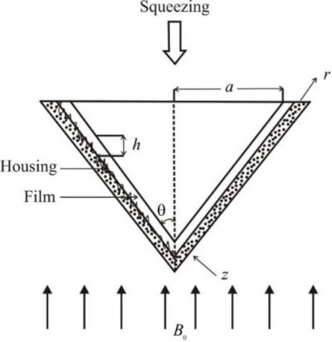
Figure 1 indicates the configuration of rough conical bearings in the existence of a transverse magnetic field. In this figure the thickness of fluid film between the plates is h. The magnetic field $B_0$ is applied along the z-direction. In the film area, micropolar fluid is taken into consideration as the lubricant. where u and v are the velocity components in r and z direction, $v_1$ is the micro-rotational velocity and $\sigma$ represents the electrical conductivity of the fluid. The parameter $\mu$ is the viscosity parameter of the base fluid as in the case of the Newtonian fluids, $\chi$ is the spin viscosity and $\gamma$ is the viscosity coefficient for micropolar fluid.
Figure 1. Configuration of the problem
The micropolar fluid equations are governed by
$\frac{1}{r} \frac{\partial(r u)}{\partial r}+\frac{\partial v}{\partial z}=0$ (1)
$\left(\mu+\frac{\chi}{2}\right) \frac{\partial^2 u}{\partial z^2}+\chi \frac{\partial v_1}{\partial z}-\sigma B_o^2 u=\frac{\partial p}{\partial r}$ (2)
$\gamma \frac{\partial^2 v_1}{\partial z^2}-\chi \frac{\partial u}{\partial z}-2 \chi v_1=0$ (3)
The relevant boundary conditions for the velocity and micro rotational velocity components are
(i) At the upper surface $z=h \sin \theta$
$u=0, v_1=0, v=\frac{d(2 h) \sin \theta}{d t}$ (4)
(ii) At the lower surface $z=-h \sin \theta$
$u=0, v_1=0, v=0$ (5)
These are the usual no-slip condition on velocity components for micropolar fluid. where the film height is h in the direction of the cone axis, the cone angle is $2 \theta$ and radius units a. The inner cone moves toward the housing with a squeezing velocity, $v_{\mathrm{sq}}=\frac{-d(2 h)}{d t} \sin \theta$ .
Eliminating $v_1$ from Eq. (2). and (3) gives
$\frac{\partial^4 u}{\partial z^4}-\xi_1 \frac{\partial^2 u}{\partial z^2}+\xi_2 u=f_1$ (6)
$\xi_1=\frac{4 \mu \chi+2 \sigma B_o^2}{\gamma(2 \mu+\chi)}, \xi_2=\frac{4 \chi \sigma B_o^2}{\gamma(2 \mu+\chi)} f_1=\frac{-4 \chi}{\gamma(2 \mu+\chi)} \frac{\partial p}{\partial r}$
To derive expression for u, integrate Eq. (6) and apply relevant velocity boundary conditions Eqns. (4)-(5) which gives,
$u=-\frac{\partial p}{\partial r} \frac{g_1-g_2}{\sigma B_o^2 g_3}$ (7)
$g_1=\varphi_2 \sinh \left(k_2 h \sin \theta\right)\left[\cosh \left(k_1 h \sin \theta\right)-\cosh \left(k_2 h \sin \theta\right)\right]$$g_2=\varphi_1 \sinh \left(k_1 h \sin \theta\right)\left[\cosh \left(k_2 h \sin \theta\right)-\cosh \left(k_2 h \sin \theta\right)\right]$$g_3=\left[\begin{array}{l}\varphi_2 \sinh \left(k_2 h \sin \theta\right) \cosh \left(k_1 h \sin \theta\right) \\ -\varphi_1 \sinh \left(k_1 h \sin \theta\right) \cosh \left(k_2 h \sin \theta\right)\end{array}\right]$
$k_1=\frac{\sqrt{\xi_1+\sqrt{\xi_1^2-4 \xi_2}}}{2}, k_2=\frac{\sqrt{\xi_1-\sqrt{\xi_1^2-4 \xi_2}}}{2}, \varphi_1=\frac{2 \sigma B_o^2-(2 \mu+\chi) k_1^2}{2 \chi k_1},\varphi_2=\frac{2 \sigma B_o^2-(2 \mu+\chi) k_2^2}{2 \chi k_2}$
The Reynolds equation for conical bearings derived by integrating the Eq. (1) and using the respective boundary conditions Eqns. (4)-(5)
$\frac{1}{r} \frac{d}{d r}\left\{f(H, N, L, M, \theta) r \frac{d p}{d r}\right\}=\frac{d H \sin \theta}{d t}$ (8)
where,
$f(H, N, L, M, \theta)=\frac{G_1-G_2}{\sigma B_0^2 k_1 k_2 G_3}$$G_1=k_1 \varphi_2 \sinh \left(k_2 h \sin \theta\right)\left[\begin{array}{l}k_1 h \sin \theta \cosh \left(k_1 h \sin \theta\right) \\ -\sinh \left(k_1 h \sin \theta\right)\end{array}\right]$$G_2=k_1 \varphi_1 \sinh \left(k_1 h \sin \theta\right)\left[\begin{array}{l}k_2 h \cosh \left(k_2 h \sin \theta\right) \\ -\sinh \left(k_2 h \sin \theta\right)\end{array}\right]$$G_3=\left[\begin{array}{l}\varphi_2 \sinh \left(k_2 h \sin \theta\right) \cosh \left(k_1 h \sin \theta\right) \\ -\varphi_1 \sinh \left(k_1 h \sin \theta\right) \cosh \left(k_2 h \sin \theta\right)\end{array}\right]$
For mathematical modeling of surface roughness, the stochastic film thickness H which consist of two parts represented as $H=h(t)+h_s(r, \theta, \xi)$ is considered.
The probability density function given by $f\left(h_s\right)$, where h(t) represents nominal smooth part of the film thickness, $h_s$ denote the random part resulting from the surface roughness asperities measured from the nominal level and $\xi$ is an index describing the definite roughness arrangements.
Using Christensen [5]
$f\left(h_s\right)=\left\{\begin{array}{cc}\frac{35}{32 c^7}\left(c^2-h_s^2\right)^3 & -c \leq h_s \leq c \\ 0 & \text { otherwise }\end{array}\right.$ (9)
where, $\bar{\sigma}=\frac{c}{3}$ is the standard deviation.
The expectancy operator is denoted as $E(*)$ and defined by
$E(*)=\int_{-\infty}^{\infty}(*) f\left(h_s\right) d h_s$ (10)
According to the stochastic theory of Christensen, two types of one-dimensional surface roughness patterns are analyzed respectively radial roughness pattern and azimuthal roughness pattern. We obtain the stochastic modified Reynolds equation on taking the average of Eq. (8) with respect to $f\left(h_s\right)$.
$\frac{1}{r} \frac{d}{d r}\left\{F\left(H^*, N, L, M, \theta\right) r \frac{d E(p)}{d r}\right\}=\frac{d H \sin \theta}{d t}$
Radial Roughness Pattern
According to the stochastic theory of Christensen, two types of one-dimensional surface roughness patterns are analyzed, respectively, radial roughness pattern and azimuthal roughness pattern. The roughness structure has the form of long, narrow ridges and valleys running in the r-direction (i.e., they are straight ridges and valley passing through z = 0, r = 0 to form star pattern), in the case the film thickness takes the form: $H=h(t)+h_s(\theta, \xi)$.
The stochastic modified Reynolds equation becomes
$\frac{1}{r} \frac{d}{d r}\left\{E[f(H, N, L, M, \theta)] r \frac{d E(p)}{d r}\right\}=\frac{d h}{d t} \sin \theta$ (12)
Azimuthal Roughness Pattern
The structure for the one-dimensional azimuthal roughness pattern on the bearing surface has the roughness structure in the form of narrow ridges and valley running in $\theta$ -direction (i.e., they are circular ridges and valley on the flat plates that are concentric on $z=0, r=0$). In this case the film thickness takes the form $H=h(t)+h_s(r, \xi)$.
$\frac{1}{r} \frac{d}{d r}\left\{\frac{1}{E[f(H, N, L, M, \theta)]^{-1}} r \frac{d E(p)}{d r}\right\}=\frac{d h}{d t} \sin \theta$ (13)
Eq. (12) and (13) together can be expressed as
$\frac{1}{r} \frac{d}{d r}\left\{r \frac{d E(p)}{d r}\right\}=\frac{-12}{F\left(H^*, N, L, M, \theta\right)} \frac{d H \sin \theta}{d t}$ (14)
where,
$F\left(H^*, N, L, M, \theta\right)=\left\{\begin{array}{l}E[f(H, N, L, M, \theta)] \text { for radial } \\ E[1 / f(H, N, L, M, \theta)]^{-1} \text { for azimuthal }\end{array}\right.$$E[f(H, N, L, M, \theta)]=\frac{35}{32 c^7} \int_{-c}^c\left(c^2-h_s^2\right)^3 f(H, N, L, M, \theta) d h_s$$E\left[\frac{1}{f(H, N, L, M, \theta)}\right]=\frac{35}{32 c^7} \int_{-c}^c \frac{\left(c^2-h_s^2\right)^3}{f(H, N, L, M, \theta)} d h_s$
The pressure boundary conditions are:
$\frac{d p}{d r}=0$ at $r=0$ (15)
$p=0$ at $r=a \operatorname{cosec} \theta$ (16)
Introducing the non-dimensionless variables and parameters
$F\left(H^*, N, L, M, \theta\right)=\frac{24\left(G_1-G_2\right)}{M^2 k_1^* k_2^* G_3}$
$G_1=\left(\begin{array}{l}0.5 k_1^* H^* \sin \theta \cosh \left(0.5 k_1^* H^* \sin \theta\right) k_2^* \varphi_2^* \sinh \left(0.5 k_2^* H^* \sin \theta\right) \\ -\sinh \left(0.5 k_1^* H^* \sin \theta\right) k_2^* \varphi_2^* \sinh \left(0.5 k_2^* H^* \sin \theta\right)\end{array}\right)$
$G_2=\left(\begin{array}{l}0.5 k_2^* H^* \sin \theta \cosh \left(0.5 k_2^* H^* \sin \theta\right) k_1^* \varphi_1^* \sinh \left(0.5 k_1^* H^* \sin \theta\right) \\ -\sinh \left(0.5 k_2^* H^* \sin \theta\right) k_1^* \varphi_1^* \sinh \left(0.5 k_1^* H^* \sin \theta\right)\end{array}\right)$
$\begin{aligned} G_3= & \varphi_2^* \sinh \left(0.5 k_2^* H^* \sin \theta\right) \cosh \left(0.5 k_1^* H^* \sin \theta\right) \\ & -\varphi_1^* \sinh \left(0.5 k_1^* H^* \sin \theta\right) \cosh \left(0.5 k_2^* H^* \sin \theta\right)\end{aligned}$
$\varphi_1^*=\varphi_1 H_0=\frac{M^2\left(1-N^2\right)-k_1^{* 2}}{2 N^2 k_1^{* 2}}$,
$\varphi_2^*=\varphi_2 H_o=\frac{M^2\left(1-N^2\right)-k_2^{* 2}}{2 N^2 k_2^{* 2}}$,
$k_1^*=k_1 H_0=\frac{\sqrt{\xi_1^*+\sqrt{\xi_1^{* 2}-4 \xi_2^*}}}{2}$,
$k_2^*=k_2 H_o=\frac{\sqrt{\xi_1^*-\sqrt{\xi_1^{* 2}-4 \xi_2^*}}}{2}$,
$\xi_1^*=\xi_1 H_o=\frac{N^2+M^2\left(1-N^2\right) L^2}{L^2}, \xi_2^*=\xi_2 H_o=\frac{N^2 M^2}{L^2}$
$H^*=\frac{H+h_s}{H_o}, N=\left(\frac{\chi}{2 \mu+\chi}\right)^{1 / 2}, L=\frac{(\gamma / 4 \mu)^{1 / 2}}{H_o}$,
$M=B_o H_o\left(\frac{\sigma}{\mu}\right)^{1 / 2}, H=\frac{2 h}{H_o}, \quad C=\frac{c}{H_o}$ and $r^*=\frac{r}{a \operatorname{cosec} \theta}$
Solution of Eq. (14) using boundary conditions
$\frac{d p^*}{d r^*}=0 \quad$ and $p^*=0, r^*=1$ (17)
gives the non-dimensional pressure equation as
$P^*=\frac{H_o^3 E(p)}{\mu\left(-\frac{d H}{d t}\right) a \operatorname{cosec} \theta}=\frac{-3\left(r^2-1\right)}{F\left(H^*, N, L, M, \theta\right)}$ (18)
The load carrying capacity equation considering the roughness effect is obtained as
$E(w)=2 \pi \int_{a \operatorname{cosec} \theta}^0 E(p) r d r$ (19)
The non-dimensional rough load carrying capacity equation is given by
$W^*=\frac{-H_o^3 E(w)}{\mu \frac{d H}{d t} a^4 \operatorname{cosec}^2 \theta}=\frac{3 \pi}{2 F\left(H^*, N, L, M, \theta\right)}$ (20)
The dimensionless time equation is given by
$T^*=\frac{-H_o^2 E(w)}{\mu a^4 \operatorname{cosec}^2 \theta}=\int_{h_j}^1 \frac{3 \pi}{2 F\left(H^*, N, L, M, \theta\right)} d H^*$ (21)
The analysis of the roughness with MHD using micropolar fluid between conical bearings is evaluated with regard to the Hartmann parameter M and roughness parameter C. The viscosity of the base fluid as in the case of the Newtonian fluid is represented as $\mu$. The spin viscosity is $\chi$ and the viscosity coefficient for micropolar fluids is $\gamma$. These viscosity parameters are grouped in the form of two parameters, the non-Newtonian coupling parameter N, the fluid-gap interacting parameter L.
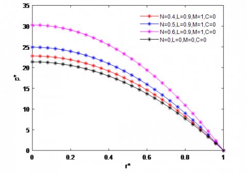
Figure 2 describes variation on pressure $p^*$ with distance in $r *$ direction for different values of N with L = 0.9, M = 1, $H^*=0.6, \theta=\frac{\pi}{3}, C=0$ when N = 0, L = 0 and M = 0 the dimensionless Reynolds equation reduces to Newtonian and non-electrically conducting case of Hamrock [14] which is given by $F=H^{* 3}$. It is noted that compared to the Newtonian the non-Newtonian micropolar fluids produces greater squeeze film pressure.
Figure 2. Variation with r* for different values of N on dimensionless pressure $p^*$ with H* = 0.6, $\theta=\frac{\pi}{3}$
Figure 3. Variation with $r^*$ for different values of M on dimensionless pressure $p^*$ with L= 0.9, H* = 0.5, $\theta=\frac{\pi}{2}$, N =0.6, C = 0.4
Figure 4. Variation with r* for different values of M on dimensionless pressure p* with L= 0.9, H* = 1.2, $\theta=\frac{\pi}{2}$, N =0.9
Figure 5. Variation with $r^*$ for different values of L on dimensionless pressure with M = 1, H* = 0.4, $\theta=\frac{\pi}{2}$, N = 0.6, C = 0.2
Figure 6. Variation with height $H^*$ for different values of N on load carrying capacity $\mathcal{W}^*$ with L = 0.9, $\theta=\frac{\pi}{6}$, N = 0.9, C = 0.4, M = 2
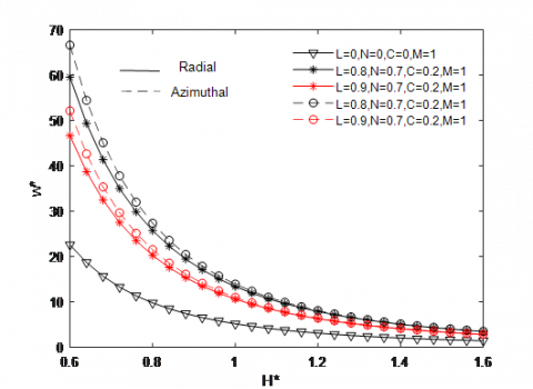
Figure 7. Variation with height $H^*$ for different values of L on load carrying capacity $\mathcal{W}^*$ with $\theta=\frac{\pi}{2}$
Figure 8. Variation with height $H^*$ for different values of $\theta$ on load carrying capacity $\mathcal{W}^*$ with L = 0.8, N = 0.7, C = 0.2, M = 1
Figure 9. Variation with $h_f$ for different values of N on time $T^*$ with L = 0.7, $\theta=\frac{\pi}{6}$, C = 0.2, M = 2
Figure 10. Variation with $h_f$ for different values of M on time $T^*$ with $\theta=\frac{\pi}{4}$
Figure 3 describes variation on pressure $p^*$ with distance in $r^*$ direction for different values of M with N = 0.6, $\theta=\frac{\pi}{2}$, H* = 0.5, C = 0.4, L =0.9. It is noted that the pressure is more prominent in the presence of a transverse magnetic field. This is because, in the case of radial roughness pattern, the roughness patterns are in the form of long narrow ridges and valleys running in the $\theta$ - direction which blocks the flow of the lubricant, while in the case of azimuthal roughness pattern, the roughness patters are in the form of long narrow ridges and valley running in the r -direction by which the lubricant can escape easily.
Figure 4 describes variation on pressure $p^*$ with rdistance in $r^*$ direction for different values of M with $\mathrm{N}=0.9$, $\theta=\frac{\pi}{2}, H^*=1.2, M=2, \mathrm{~L}=0.9 \quad$ for $\quad N \neq 0, L \neq 0, M=0$ and C=0. When M=0 the equation reduces to non- Newtonian and non- electrically conducting case of Prakash and Shina [15] which is given by $F=H^{* 3}+12 L^2 H^*-6 N L H^{* 2} \operatorname{coth}\left(\frac{N H^*}{2 L}\right)$. It is observed that compared to the non-magnetic case the magnetic case is more pronounced for pressure.
Figure 5 describes variation of pressure with $r^*$ for different values of L on dimensionless pressure with M = 2, $H^*=0.4, \theta=\frac{\pi}{2}, N=0.6, \mathrm{C}=0.1$. The pressure decreases for increasing values of fluid gap interaction parameter L.
Figure 6 describes variation with height $H^*$ on load carrying capacity $w^*$ for different parameter values of coupling number N. The load carrying capacity $w^*$ increases for increasing value of coupling number N.
Figure 7 describes variation on load carrying capacity $w^*$ as a function of $H^*$ for different values of L with$\theta=\frac{\pi}{2}, M=1$, $\mathrm{N}=0.7, \mathrm{C}=0.2$. It shows that the for$N=0, L=0, \mathrm{C}=0$ and $M \neq 0$ the equation reduces to Newtonian and electrically conducting case obtained by Lin [16] which is given by. $F=\frac{12 M H^*-24 \tanh \left(0.5 M H^*\right)}{M^3}$ . The results of non-Newtonian case is enhanced when compared with the electrically conductive Newtonian case.
Further it is noticed that the effect of azimuthal roughness is to increase the load carrying capacity for all values of the fluid-gap interacting parameter L whereas radial roughness causes a decrease in load as compared to the smooth case. Thus, the surface roughness effects are strongly dependent on surface texture. One type of texture may have just an opposite influence as compared to another. The effect caused by azimuthal roughness can be treated as the one produced in the opposite direction of radial roughness.
Figure 8 describes variation on load carrying capacity $w^*$ as a function of $H^*$ for varying values of $\theta$ with M = 1, L = 0.8, C = 0.2, N = 0.7 The dimensionless load carrying capacity $w^*$ increases with the increasing value of $\theta$.
Figure 9 displays that the variation of $h_f$ with time T* for various values of N with $\theta=\frac{\pi}{6}, M=2, \mathrm{~L}=0.8, C=0.3$. The time increases(decreases) with the increasing value of N for the azimuthal(radial) roughness pattern.
The variation of $h_f$ with time T* for varying values of M with $\theta=\frac{\pi}{2}$ is shown in given Figure 10. It is noted that existence of roughness and applied magnetic field increases the squeezing time compared to the smooth surface.
In this paper, the impact of roughness with MHD between the conical bearings using micropolar fluid is analyzed. The conclusions are obtained according to the numerical computations.
|
Bo |
Strength of applied magnetic field |
|
M |
Hartmann number = $\left(B_0 h_0\left(\frac{\sigma}{\mu}\right)^{1 / 2}\right)$ |
|
h |
Film thickness |
|
H* |
Non-dimensional film thickness |
|
u, v |
Velocity components in r and z direction |
|
v1 and v2 |
Components of micro rotational velocity |
|
Greek symbols |
|
|
$\sigma$ |
Electrical conductivity |
|
$\chi$ |
Spin viscosity |
|
$\mu$ |
Newtonian viscosity |
|
$\gamma$ |
Viscosity coefficient of micropolar fluid |
|
L |
Fluid-gap interacting parameter |
|
C |
Roughness parameter |
|
N |
Non-Newtonian coupling parameter |
|
Subscripts |
|
|
p* |
Non-dimensional pressure |
|
w* |
Non-dimensional load carrying capacity |
|
T* |
Non-dimensional time |
[1] Eringen, A.C. (1965). Linear theory of micropolar elasticity. Journal Mathematics and Mechanics, 15: 909-923. https://doi.org/10.1512/iumj.1966.15.15060
[2] Eringen, A.C. (1966). Theory of micropolar fluids. Journal of Mathematics and Mechanics, 16: 1-16. http://dx.doi.org/10.1512/iumj.1967.16.16001
[3] Ramanaiah, G., Dubey, J.N. (1977). Optimum slider profile of a slider bearing lubricated with a micropolar fluid. Wear, 42(1): 1-7. https://doi.org/10.1016/0043-1648(77)90162-4
[4] Zaheeruddin, K.H., Isa, M. (1978). Characteristics of a micropolar lubricant in a squeeze film porous spherical bearing. Wear, 51(1): 1-10. https://doi.org/10.1016/0043-1648(78)90049-2
[5] Christensen, H., Tonder, K. (1973). The hydrodynamic lubrication of rough journal bearings. ASME Journal of Lubrication Technology, 1: 166-171. https://doi.org/10.1115/1.3451759
[6] Rajani, C.B., Hanumagowda, B.N., Shigehalli, V.S. (2018). Effects of surface roughness on conical squeeze film bearings with micropolar fluid. Journal of Physics: Conference Series, 1000(1): 01-11. https://doi.org/10.1088/1742-6596/1000/1/012079
[7] Rao, P.S., Murmu, B., Agarwal, S. (2018). Piezo-Viscous dependency and surface roughness effects on the squeeze film characteristics of non-newtonian micropolar fluid in conical bearings. Tribology, 13(5): 282-289. https://doi.org/10.2474/trol.13.282
[8] Halambi, B., Hanumagowda, B.N. (2018). Effects of surface roughness with MHD on the micro polar fluid flow between rough elliptic plates. International Journal of Mechanical Engineering and Technology, 9(11): 586-598. https://doi.org/10.17051/ilkonline.2021.04.33
[9] Lin J.R. (2003). Magneto‐hydrodynamic squeeze film characteristics for finite rectangular plates. Industrial Lubrication and Tribology. https://doi.org/10.1108/00368790310470912
[10] Hanumagowda B.N., Swapana N., Vishu Kumar, M. (2017). Effect of MHD and couple stress on conical bearing. International Journal of Pure and Applied Mathematics, 113(6). https://doi.org/10.1088/1742-6596/1000/1/012089
[11] Rao. P.S., Kumar Rahul, A. (2019). Effect of viscosity variation on non-Newtonian lubrication of squeeze film conical bearing having porous wall operating with Rabinowitsch fluid model. Proceedings of the Institution of Mechanical Engineers, Part C: Journal of Mechanical Engineering Science, 233(7): 2538-51. https://doi.org/10.1177/0954406218790285
[12] Lin. J.R., Kuo, C.C., Liao, W.H., Yang, C.B. (2012). Non-Newtonian micropolar fluid squeeze film between conical plates. Zeitschrift für Naturforschung A, 1(67): 333-337. https://doi.org/10.5560/zna.2012-0036
[13] Sangeetha, S., Govindarajan, A. (2019). Analysis of viscosity variation with MHD on circular stepped plates in couple stress fluid. Journal of Interdisciplinary Mathematics, 22(6): 889-901. https://doi.org/10.1080/09720502.2019.1688945
[14] Hamrock, B.J. (1994). Fundamentals of fluid film lubrication. McGraw-Hill New York. https://doi.org/10.1201/9780203021187
[15] Prakash, J., Sinha, P. (1976). Squeeze film theory for micropolar fluids. ASME Journal of Lubrication Technology, 96: 139-144. https://doi.org/10.1115/1.3452749
[16] Lin, J.R. (2001). Magneto-hydrodynamic squeeze film characteristics between annular disks. Industrial Lubrication and Tribology, 53(2): 66-71. https://doi.org/10.1108/00368790110384028