Bidemi Olumide Falodun* | Adeola John Omowaye | Funmilayo Helen Oyelami | Ebenezer Olubunmi Ige
© 2022 IIETA. This article is published by IIETA and is licensed under the CC BY 4.0 license (http://creativecommons.org/licenses/by/4.0/).
OPEN ACCESS
The dynamics of MHD non-Newtonian fluid flow past a cylinder with slip boundary condition and magnetic field is addressed in this study. The non-Newtonian fluid (tangent hyperbolic) considered in this study are nail polish and whipped cream. This article investigates the statistical analysis of two-dimensional MHD tangent hyperbolic fluid flow over a cylinder with slip condition. The partial differential equations describing the problem are later transformed into the ordinary differential equation by similarity variables. The derived model is solved by the spectral homotopy analysis method (SHAM). The characteristics of the parameters of the flow are demonstrated by the velocity of the flow. The skin friction coefficient is computed and presented with the aid of a tables. The slope of the linear regression is obtained through the data points while bar charts for engineering quantities of interest are presented. The findings indicated that an increase in magnetic parameters builds a resistance to the flow. Also, it was discovered that the radius of curvature decreases when the curvature parameter increases.
mass transfer, non-Newtonian fluid, MHD, cylinder slip
A non-Newtonian fluid is a class of fluid that does not follow the linear behaviour between stress and shear rate. This means that such fluid does not obey the Newton’s law of viscosity. However, the Newtonian fluids obeys the Newton’s law of viscosity. Examples of non-Newtonian fluids are tangent hyperbolic, Casson, Walters-B, power law while water and gases are examples of Newtonian fluids. It follows that any fluid of this type does not follow the law of viscosity by Newton. Meanwhile, the viscosity of a non-Newtonian fluid depends on the shear stress. However, custard, toothpaste, starch, paint, blood and shampoo are examples of non-Newtonian fluids. Also, due to recent interest in the behaviour of a non-Newtonian type of fluid, many researchers have investigated the behaviour of this type of fluid by examing the characteristics features of different physical properties. More so, the hydrodynamic impact of inclination on tangent hyperbolic flow was considered by Ali et al. [1]. Bilal et al. [2] examined Williamson fluid with nanofluid pasted on a stretch sheet. Khan et al. [3] discussed heat together with mass transport of Williamson nano fluid flow. Dawar et al. [4] did 3D Williamson nanofluid in Darcy-Forhheimer porous medium. Lund et al. [5] considered MHD flow of Williamson fluid with slippage. It was shown that a dual solution exists. The upper converted maxwell fluid with varied thermo-physical conditions was examined by Omowaye and Animasaun [6]. Omowaye et al. [7] discussed Dufour and Soret on steady MHD convection flow with temperature-dependent viscosity using homotopy analysis. Fagbade et al. [8] work was centred on MHD free convection flow of viscoelastic fluid with thermal radiation and heat source or sink by SHAM. While Falodun and Omowaye [9] addressed the problem of double-diffusive magnetohydrodynamics (MHD) non-Darcy convective flow of heat embedded in a thermally-stratified porous medium.
MHD explains the behaviour of flow in an electrically conducting fluid existing in magnetic and electric field. An induced current polarizes the electrically conducting fluid and posed changes to the imposed magnetic field. The induced current due to an electrically conducting fluid flow because of magnetic field gives rise to a resistive force (Lorentz) and retards the motion of fluid. The phenomenon of MHD finds applications in astrophysics, petrochemical industry, heat exchanger design and geophysics. The tangent hyperbolic model is commonly used in defining and predicting shear thinning. Many authors had explored the model of tangent hyperbolic with different physical properties. This type of fluid is mostly used in laboratory experiments. It is an important fluid model in industry as well as biology. Examples are Ketchup, melts, paint, polymers and blood. Patil et al. [10] examined dissipation together with the convective condition on tangent hyperbolic fluid. Hussain et al. [11] examined MHD tangent hyperbolic fluid and the effects of viscous dissipation on it. The tangent hyperbolic flow in nanoparticles and magnetohydrodynamics was discussed by Ibrahim [12]. Kumar et al. [13] addressed the squeezed flow of unsteady tangent hyperbolic fluid past a sensor surface by varying thermal conductivity. The study of exponentially vertical stretched cylinder of tangent hyperbolic fluid flow in a boundary layer was proposed by Naseer et al. [14]. The transport of dusty fluid in hyperbolic tangent flow past a stretching sheet together with heat transfer was done by Kumar et al. [15]. The major reason why we embark on this research is to examine MHD tangent hyperbolic flow over a cylinder together with slip boundary condition.
This paper addressed the dynamics of MHD non-Newtonian (tangent hyperbolic) fluid past a cylinder with slip boundary condition and magnetic field. No studies have examined this type of problem in literature to the best of our knowledge. Keeping this in mind, this study is set to explore the dynamics of MHD tangent hyperbolic fluid past a cylinder with slip boundary condition numerically. The examples of tangent hyperbolic fluid considered are nail polish and whipped cream. This study is an extension of the published work of Malik et al. [16]. These fluids find application in industrial engineering and industries where cream is produced. Based on these applications, this research is of great importance to engineers and scientist. A hybrid spectral method combining the concept of Chebyshev spectral collocation and homotropy analysis method was utilized to solved the system of equations. The significance of pertinent flow parameters is illustrated graphically while numerical computations of engineering quantities of interest are tabulated. The outcomes of this study were compared with other results in literature and was found in excellent agreement. This paper is organized as follows: section 1 comprises of introduction, section 2 comprises of mathematical analysis, the numerical procedures are presented in section 3. The results and discussion are presented in section 4 while the conclusion of findings in section 5.
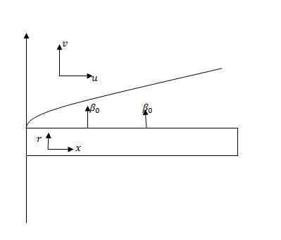
A flow that is steady, incompressible, laminar and two dimensional MHD tangent hyperbolic fluid over a cylinder together with slip boundary condition is considered. The x-direction is along the cylinder and the y is perpendicular to it, this is shown in Figure 1 below. A magnetic field $\left(B_0\right)$ which has uniform strength is applied in a normal direction to the flow. Akbar et al. [17] explained constitutive equation for the hyperbolic flow as
$\tau=\left[\mu_{\infty}+\left(\mu_0+\mu_{\infty}\right) \tanh (\Gamma \dot{\gamma})^n\right] A_1$ (1)
where, $\mu_{\infty}$ is the infinite shear rate viscosity, $\mu_0$ is the zero shear rate viscosity, $\Gamma$ is the dependent material constant, n is the power law index or flow behavior index, $A_1$ is the first Rivlin-Erickson tensor and $\dot{\gamma}$ is given as
$\dot{\gamma}=\sqrt{\frac{1}{2} \operatorname{tr}\left(A_1^2\right)}$ (2)
For the sake of simplicity in this paper, we assume $\mu_{\infty}=0$ in Eq. (1) and $\Gamma \dot{\gamma}<1$ which is the tangent hyperbolic fluid, it explains the shear thinning phenomena. Implementing all the above in Eq. (1) to obtain
$\tau=\mu_0\left[(\Gamma \dot{\gamma})^n\right] A_1$ (3)
After simplication, the above becomes
$\tau=\mu_0[1+n(\Gamma \dot{\gamma}-1)] A_1$ (4)
Figure 1. The coordinate of the flow
Also, the assumption of no slip condition on the cylinder is no longer valid in the flow rather the flow is under the influence of surface slip condition. Invoking the boundary layer approximation then, (Motsa [18]) the flow is governed by the following equations:
$u \frac{\partial u}{\partial x}+v \frac{\partial u}{\partial r}=0$ (5)
$\begin{aligned} u \frac{\partial u}{\partial x}+v \frac{\partial u}{\partial x}=v[ & {[1-n) \frac{\partial^2 u}{\partial r^2}+(1-n) \frac{1}{r} \frac{\partial u}{\partial r} } \\ & \left.+n \sqrt{2} \Gamma \frac{\partial u}{\partial r} \frac{\partial^2 u}{\partial r^2}+\frac{n \Gamma}{\sqrt{2} r}\left(\frac{\partial u}{\partial r}\right)^2\right] \\ & -\frac{\sigma \beta_0^2}{\rho} u\end{aligned}$ (6)
The boundary conditions are:
$u=U_w(x)+L \frac{\partial u}{\partial r} v=0$ at $r=R$
$u \rightarrow U_{\infty}(x)=0, \quad$ as $r \rightarrow \infty$ (7)
where, u and v are the velocity along x and r-axes, v is kinematic viscosity, n is the power law index, $\Gamma$ is the Williamson parameter, $\sigma$ is the electrical charge density, $\beta_0$ is the magnetic field, $\rho$ is the density, $L$ is the slip length, $U_w(x)$ is the stretching velocity, $U_{\infty}(x)$ is the free stream velocity and $U_w(x)$ is given as $\frac{a x}{L}$ where L is the characteristics length and $L$ is positive constant.
The following similarity variables are considered in transforming Eqns. (5)-(7).
$\eta=\sqrt{\frac{a}{L v}}\left(\frac{r^2-R^2}{2 R}\right), \phi=\sqrt{\frac{v a}{L}} R f(\eta) x, u=\frac{1}{r} \frac{\partial \phi}{\partial r}, v=-\frac{1}{r} \frac{\partial \phi}{\partial x}$ (8)
then Eqns. (5)-(7) become
$(1-n)(1+2 k \eta) f^{\prime \prime}+f f^{\prime \prime}-\left(f^{\prime}\right)^2+2 k(1-n) f^{\prime \prime}+2 \lambda n(1+2 k \eta)^{\frac{3}{2}} f^{\prime \prime} f^{\prime \prime \prime}+3 \lambda k(1+2 k \eta)^{\frac{1}{2}}\left(f^{\prime \prime}\right)^2-M^2 f^{\prime}=0$ (9)
The transformed boundary conditions are
$f(0)=0, f^{\prime}(0)=1+s f^{\prime \prime}(0)$, as $\eta=0$ (10)
$f^{\prime}(\infty) \rightarrow 0$ as $\eta \rightarrow \infty$ (11)
where, $k=\left(\frac{1}{R}\right) \sqrt{\frac{v L}{a}}$ is the curvature parameter, $\lambda=\frac{\Gamma a^3 x}{\sqrt{2 v} L^{\frac{3}{2}}}$ is the dimensionless Weissenberg number, $M^2=\frac{\sigma \beta_0^2 L}{\rho a}$ is the Hartmann number and $S=\frac{a^{\frac{3}{2}} r L}{L^{\frac{3}{2}} v^{\frac{1}{2}}}$ is the slip parameter.
The fluid drag is given as
$C_f=\frac{\tau_w}{\frac{\rho a^2 x^2}{2 L^2}}$ where $\tau_w=\mu\left((1-n) \frac{\partial u}{\partial r}+\frac{2}{\sqrt{2}} \Gamma\left(\frac{\partial u}{\partial r}\right)^2\right)_{r=R}$
The dimensionless form is
$C_f R e_x^{\frac{1}{2}}=(1-n) f^{\prime \prime}(0)+n \lambda f^{\prime \prime 2}$ where $\operatorname{Re}_x^{\frac{1}{2}}=\frac{a^{\frac{1}{2}} x}{v^{\frac{1}{2}} L^{\frac{1}{2}}}$
The solution procedures to the problem are highlighted in this part of the work. The flow equation of this problem is solved numerically using pseudospectral homotopy analysis method (SHAM). SHAM is the combination of the procedure of Chebyshev pseudospectral method and the well known homotopy analysis method (HAM). SHAM was proposed by Motsa [18] and is used to decomposed the systems of nonlinear equations by defining an algebraic transformation given as in Fagbade et al. [8]
$\xi=\frac{2 \eta}{L}-1, \xi \in[-1,1], f(\eta)=f(\xi)+f_0(\eta)$ (12)
The method requires the domain to be transformed from [0, L] to [−1, 1] by the mapping defined in Eq. (12). Hence, substituting Eq. (12) into the transformed nonlinear Eq. (9) to obtain
$\begin{aligned}(1-n)\left(1_k \eta\right) f^{\prime \prime} & +f f^{\prime \prime}+a_1 f+a_2 f^{\prime \prime}-f^{\prime} f^{\prime}+a_3 f^{\prime} \\ & +2 k(1-n) f^{\prime \prime}+2 \lambda n(1 \\ & -2 k \eta)^{\frac{3}{2} f^{\prime \prime} f^{\prime \prime \prime}}+a_4 f^{\prime \prime}+a_5 f^{\prime \prime \prime} \\ & +3 \lambda k(1+2 k \eta)^{\frac{1}{2}} f^{\prime \prime} f^{\prime \prime}+a_6 f^{\prime \prime} \\ & -M^2 f=H_1(\eta)\end{aligned}$ (13)
where the coefficient parameters in the above equation are
$a_1=f^{\prime \prime}{ }_0, a_2=f_0, a_3=-2 f_0^{\prime}, a_4=2 \lambda n(1-2 k \eta)^{\frac{3}{2}} f^{\prime \prime \prime}{ }_0, a_5=2 \lambda n(1-2 k \eta)^{\frac{3}{2}} f^{\prime \prime}{ }_0, a_6=6 \lambda k(1-2 k \eta)^{\frac{3}{2}}$$H_1(\eta)=-(1-n)(1-2 k \eta)^{\frac{3}{2}} f^{\prime \prime}{ }_0-f_0 f^{\prime \prime}{ }_0+f^{\prime}{ }_0 f^{\prime}{ }_0-2 k(1-n) f^{\prime \prime}{ }_0-2 \lambda n(1-2 k \eta)^{\frac{3}{2}} f^{\prime \prime}{ }_0 f^{\prime \prime \prime}-3 \lambda k(1-2 k \eta)^{\frac{1}{2}} f^{\prime \prime}{ }_0 f^{\prime \prime}{ }_0+M^2 f^{\prime}{ }_0$
The appropriate boundary conditions to Eq. (10) are
$f(-1)=f(1)=0, f^{\prime}(-1)=f^{\prime}(1)=0$ (14)
With the concept of SHAM, we chose an initial approximation given as:
$f_0(\eta)=\left(e^{-\eta}-1\right)\left(\frac{1}{1+s f^{\prime \prime}(0)}\right)+\eta$ (15)
The initial approximation above must satisfy the boundary conditions (10) and (11). The linear part of Eq. (13) is given as:
$(1-n)(1+k \eta) f^{\prime \prime}+a_2 f+a_2 f^{\prime \prime}+a_3 f^{\prime}+2 k(1-n) f^{\prime \prime}+a_4 f^{\prime \prime}+a_5 f^{\prime \prime \prime}+a_6 f^{\prime \prime}-M^2 f^{\prime}=H_1(\eta)$ (16)
We proceed to apply the Chebyshev pseudospectral method on the Eq. (12) above and the unknown function $f(\xi)$ is defined as
$f(\xi)=\sum_{k=0}^N f_k T_k$
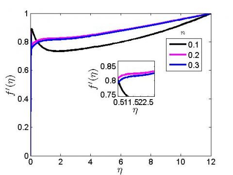
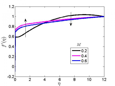
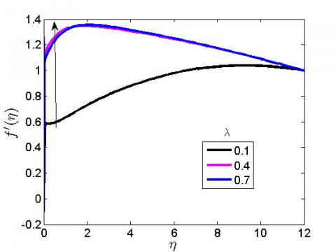
This section demonstrates the influences of the physical parameters on the flow of hyperbolic fluid flow over a stretching cylinder with slip boundary condition. These are the parameters of the flow, the Hartmann number (M), curvature parameter (k), Weissenberg number (λ), power-law index (n), and slip parameter (s). The parametric values in the literature guided in arriving at the values of the parameters chosen in plotting the graphs. The various values chosen are illustrated in the legend of the graphs. Also, the results of the computations for various parameters of the flow are presented in graphs and tables. The effects of a power-law index on the flow is shown in Figure 2. It can be seen that the velocity increases on the cylinder as the fluid moves away from the cylinder, towards the free stream the velocity decreases. This agrees with Malik et al. [16]. In Figure 3, we noticed that at the initial point on the cylinder the velocity increased to a certain point as it moves away from the cylinder and there was a cross-over of the profiles. From this point, the velocity decreases when the Hartmann number (M) increases. Hence, this enhances the Lorentz force which builds up a resistance to the flow field, and this decreases the velocity. Figure 4 illustrates the effects of the Weissenberg number λ on the flow velocity. Obviously, velocity increases after the Weissenberg number increases. This happens because the relaxation time increases which enhances the flow and hence the velocity increases.
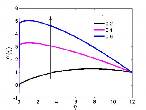
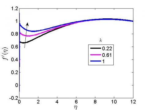
The influence of the slip parameter on the velocity of the fluid as it flows on the cylinder is illustrated in Figure 5. An increase in slip parameter accounts for the increase in the velocity of the fluid. This happens because of the slip condition on the surface of the cylinder. Hence, the fluid adjacent to the surface of the cylinder permits an influx of fluid to slide on the surface. This shows that, an increase in the slip parameter leads to higher increase in the thickness of the hydrodynamic fluid layer which allows fluid flow at the surface of the cylinder. However, the fluid accelerates for a distance close to the surface of the cylinder. This is confirmed by the fact that higher means an increase in lubrication and slipperiness of the surface. Figure 6 depicts curvature parameter influence on the velocity of the flow. Obviously, velocity increases when the curvature parameter increases. This can be explained as when the curvature parameter is increased this makes the cylinder radius of curvature decrease which in turn causes the area of the cylinder to decrease. Hence, the velocity of the fluid increases as shown in Figure 6.
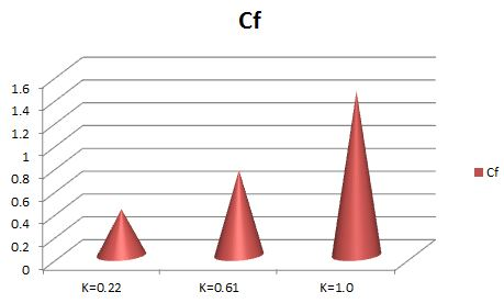
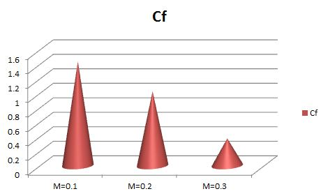
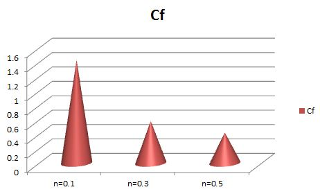
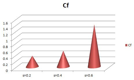
Figure 7 shows the impact of the curvature parameter (K) on the local skin friction. the curvature parameter is the ratio of the boundary layer thickness and radius of the cylinder. Physically, as the curvature parameter increase (i.e K=0.22, K=0.61, and K=1.0), the local skin friction within the cylinder is observed to increase. This shows that when K=0.22 the local skin friction is 0.2m/s when K=0.61 the local skin friction is 0.60m/s while at K=1.0 the local skin friction is 1.28m/s. Figure 8 shows the impact of Hartmann number (M) on the local skin friction. When M=0.1 the local skin friction within the cylinder is 1.3m/s. When M=0.2 the local skin friction is observed to be 0.9m/s and when M=0.3 the local skin friction is noticed to be 0.21m/s. The result in Figure 8 shows that as the Hartmann number increases the local skin friction within the boundary layer reduces. Therefore, an increase in M decreases the thickness of the hydrodynamic boundary layer. Figure 9 shows the impact of the power-law index (n) on the local skin friction. For n=0.1 the local skin friction is noticed to be 1.3m/s, for n=0.3 the local skin friction is noticed to be 0.41m/s while for n=0.5 the local skin friction is observed to be 0.22m/s. This implies a decrease in the thickness of the hydrodynamic boundary layer for an increase in the power-law index. Figure 10 indicates the effect of the slip parameter on the local skin friction. Physically, when s=0.2 the local skin friction is noticed to be 0.21m/s, when s=0.4 the local skin friction is observed to be 0.41m/s. Also, when s=0.6 the local skin friction is noticed to be 1.23m/s. This implies that an increase in slip parameter increases the hydrodynamic boundary layer thickness.
In Table 1, it is observed that the skin friction reduces at the rate of -5.3155 as the magnetic parameter increases while skin friction increases at the rate of 1.6575167 as the Weissenberg number increases in Table 2. Table 3 is in terms of curvature parameters. An increase in curvature parameter in Table 3 shows an increase in the local skin friction at the rate of 1.328077. In Table 3, an increase in the curvature parameter is found to enhance the fluid flow in the hydrodynamic boundary layer. Hence, the fluid particles move very fast within the cylindrical pipe. In Table 4, a higher value of the power law index (n) is observed to slow down the motion of the fluid. As the value of power law index increases the more, the skin friction coefficient decreases at the rate of -2.53225. In Table 5, a higher value of the slip parameter is discovered to enhance the thickness of the hydrodynamic boundary layer by increasing the skin friction. In Table 4, increase in the power law index is observed to gradually decrease the skin friction. However, the slope of linear regression decrease is -2.53225. Also, in Table 5 as the slip parameter increases, the skin friction is observed to increase. This increase hereby leads to slope of linear regression of -0.036. The present analysis was compared with the existing work of Malik et al. [16] in Table 6. The outcomes in the present analysis were found to be in good agreement with that of Malik et al. [16] as shown in Table 6.
Table 1. Computational values for skin-friction coefficient Cf with variation of magnetic parameter
|
M |
Cf |
|
0.1 |
1.4368 |
|
0.2 |
1.0256 |
|
0.3 |
0.37387 |
|
$S_{l p}$ |
-5.3155 |
Table 2. Computational values for skin-friction coefficient Cf with variation of Weissenberg number
|
$k$ |
Cf |
|
0.1 |
0.4359 |
|
0.4 |
0.4373 |
|
0.7 |
1.4410 |
|
$S_{l p}$ |
1.6575167 |
Table 3. Computational values for skin-friction coefficient $C f$ with variation of curvature parameter
|
k |
Cf |
|
0.22 |
0.4018 |
|
0.61 |
0.7451 |
|
1.0 |
1.4377 |
|
$S_{l p}$ |
1.328077 |
Table 4. Computational values for skin-friction coefficient Cf with variation of Power law index
|
n |
Cf |
|
0.1 |
$1.4350$ |
|
0.3 |
$0.5855$ |
|
0.5 |
$0.4221$ |
|
$S_{l p}$ |
$-2.53225$ |
Table 5. Computational values for skin-friction coefficient Cf with variation of slip parameter
|
s |
Cf |
|
0.2 |
0.3746 |
|
0.4 |
0.5425 |
|
0.6 |
1.4206 |
|
$S_{l p}$ |
-0.036 |
Table 6. Validation of the present study with Malik et al. [16]
|
|
|
|
|
Malik et al. [16] |
Present study |
|
M |
$\lambda$ |
K |
n |
$C_f R_x^{\frac{1}{2}}$ |
$C_f R_x^{\frac{1}{2}}$ |
|
0.1 |
0.1 |
0.1 |
0.1 |
-0.9799 |
-0.9798 |
|
0.2 |
|
|
|
-0.9968 |
-0.9967 |
|
0.3 |
|
|
|
-1.0432 |
-1.0431 |
|
0.1 |
0.1 |
|
|
-0.9799 |
-0.9798 |
|
|
0.2 |
|
|
-0.9780 |
-0.9779 |
|
|
0.3 |
|
|
-0.9760 |
-0.9759 |
|
|
0.1 |
0.1 |
|
-0.9799 |
-0.9798 |
|
|
|
0.2 |
|
-1.0098 |
-1.0097 |
|
|
|
0.3 |
|
-1.0393 |
-1.0392 |
|
|
|
0.1 |
0.1 |
-0.9799 |
-0.9798 |
|
|
|
|
0.2 |
-0.9192 |
-0.9191 |
|
|
|
|
0.3 |
-0.8535 |
-0.8534 |
Figure 2. Effect of power law index on velocity profile
Figure 3. Effect of Hartmann number on velocity profile
Figure 4. Effect of Weissenberg number on velocity profile
Figure 5. Effect of slip parameter on velocity profile
Figure 6. Effect of curvature parameter on velocity profile
Figure 7. Effect of curvature parameter on velocity profile
Figure 8. Effect of Hartmann parameter on velocity profile
Figure 9. Effect of Power law index parameter on velocity profile
Figure 10. Effect of slip parameter on velocity profile
In this exploration, the statistical and numerical analysis of an electrically conducting flow of tangent hyperbolic fluid over a stretching cylinder is addressed. The flow is assumed to be under the influence of surface slip condition. The rate of change of pertinent flow parameters on the local skin friction is tabulated. The model equation is numerically solved and the influence of parameters such as curvature parameter, Weissenberg number, Hartmann number, and slip parameter are analyzed. The major findings are as follows:
The outcome of this paper finds applications in science and engineering such as MHD accelerator, polymer additives, heat exchanger device, food processing and so on.
|
$u$ and $v$ |
velocity along $x$ and $r$ -axes |
|
$\nu$ |
kinematic viscosity |
|
$n$ |
power law index |
|
$\Gamma$ |
Williamson parameter |
|
$\sigma$ |
electrical charge density |
|
$\beta_0$ |
magnetic field |
|
$\rho$ |
density |
|
L |
slip length |
|
$U_w(x)$ |
stretching velocity |
|
$U_{\infty}(x)$ |
free stream velocity |
|
$a$ |
positive constant |
[1] Ali, A., Hussain, R., Maroof, M. (2019). Inclined hydromagnetic impact on tangent hyperbolic fluid flow over a vertical stretched sheet. AIP Advances, 9: 125022. https://doi.org/10.1063/1.5123188
[2] Bilal, M., Sagheer, M., Hussain, S. (2018). Numerical study of magnetohydrodynamics and thermal radiation on Williamson nanofluid flow over a stretching cylinder with variable thermal conductivity. Alexandria Engineering Journal, 57(4): 3281-3289. https://doi.org/10.1016/j.aej.2017.12.006
[3] Khan, M., Malik, M.Y., Salahuddin, T., Hussian, A. (2018). Heat and mass transfer of Williamson nanofluid flow yield by an inclined Lorentz force over a nonlinear stretching sheet. Results in Physics, 8: 862-868. https://doi.org/10.1016/j.rinp.2018.01.005
[4] Dawar, A., Shah, Z., Islam, S., Khan, W., Idrees, M. (2019). An optimal analysis for Darcy–Forchheimer three-dimensional Williamson nanofluid flow over a stretching surface with convective conditions. Advances in Mechanical Engineering, 11(3): 1-15. https://doi.org/10.1177/1687814019833510
[5] Lund, L.A., Omar, Z., Khan, I. (2019). Analysis of dual solution for MHD flow of Williamson fluid with slippage. Heliyon, 5(3): e01345. https://doi.org/10.1016/j.heliyon.2019.e01345
[6] Omowaye, A.J., Animasaun, I.L. (2016). Upper-convected Maxwell fluid flow with variable thermo-physical properties over a melting surface situated in hot environment subjected to thermal stratification. Journal of Applied Fluid Mechanics, 9(4): 1777-1790.
[7] Omowaye, A.J., Fagbade, A.I., Ajayi, A.O. (2015). Dufour and Soret effects on steady MHD convective flow of a fluid in a porous medium with temperature dependentviscosity: Homotopy analysis approach. Journal of the Nigerian Mathematical Society, 34(3): 343-360. https://doi.org/10.1016/j.jnnms.2015.08.001
[8] Fagbade, A.I., Falodun, B.O., Omowaye, A.J. (2018). MHD natural convection flow of viscoelastic fluid over an accelerating permeable surface with thermal radiation and heat source or sink: Spectral homotopy analysis approach. Ain Shams Engineering Journal, 9(4): 1029-1041. http://dx.doi.org/10.1016/j.asej.2016.04.021.
[9] Falodun, O.B., Omowaye, A.J. (2019). Double-diffusive MHD convective flow of heat and mass transfer over a stretching sheetembedded in a thermally-stratified porous medium. World Journal of Engineering, 16(6): 712-724. https://doi.org/10.1108/WJE-09-2018-0306
[10] Patil, M., Mahesha, Raju, C.S.K. (2019). Convective conditions and dissipation on Tangent Hyperbolic fluid over a chemically heating exponentially porous sheet. Nonlinear Engineering, 8(1): 407-418. https://doi.org/10.1515/nleng-2018-0003
[11] Hussain, A., Malik, M.Y., Salahuddin, T., Rubab, A., Khan, M. (2017). Effects of viscous dissipation on MHD tangent hyperbolic fluid over a nonlinear stretching sheet with convective boundary conditions. Results in Physics, 7: 3502-3509. https://doi.org/10.1016/j.rinp.2017.08.026
[12] Ibrahim, W. (2017). Magnetohydrodynamics (MHD) flow of a tangent hyperbolic fluid with nanoparticles past a stretching sheet with second order slip and convective boundary condition. Results in Physics, 7: 3723-3731. https://doi.org/10.1016/j.rinp.2017.09.041
[13] Kumar, K.G., Gireesha, B.J., Krishanamurthy, M.R., Rudraswamy, N.G. (2017). An unsteady squeezed flow of a tangent hyperbolic fluid over a sensor surface in the presence of variable thermal conductivity. Results in Physics, 7: 3031-3036. https://doi.org/10.1016/j.rinp.2017.08.021
[14] Naseer, M., Malik, M.Y., Nadeem, S., Rehman, A. (2014). The boundary layer flow of hyperbolic tangent fluid over a vertical exponentially stretching cylinder. Alexandria Engineering Journal, 53(3): 747-750. https://doi.org/10.1016/j.aej.2014.05.001
[15] Kumar, K.G., Gireesha, B.J., Gorla, R.S.R. (2018). Flow and heat transfer of dusty hyperbolic tangent fluid over a stretching sheet in the presence of thermal radiation and magnetic field. International Journal of Mechanical and Materials Engineering, 13(2): 1-11. https://doi.org/10.1186/s40712-018-0088-8
[16] Malik, M.Y., Salahuddin, T., Hussain, A., Bilal, S. (2015). MHD flow of tangent hyperbolic fluid over a stretching cylinder: Using Keller box Method. Journal of Magnetism and Magnetic Materials, 395: 271-276. https://doi.org/10.1016/j.jmmm.2015.07.097
[17] Akbar, N.S., Nadeem, S., Haq, R.U., Khan, Z. (2013). Numerical solutions of Magnetohydrodynamic boundary layer flow of tangent hyperbolic fluid towards a stretching sheet. Indian Journal of Physics, 87(11): 1121-1124. https://doi.org/10.1007/s12648-013-0339-8
[18] Motsa, S.S. (2012). New iterative methods for solving nonlinear boundary value problems in: Fifth Annual Workshop on Computational Applied Mathematics and Mathematical Modelling in Fluid Flow, School of Mathematics, statistics and computer science, Pietermaritzburg Campus, 9-13.