Slimane Niou* | Abdessalam Otmani | Azzeddine Dekhane | Salaheddine Azzouz
© 2022 IIETA. This article is published by IIETA and is licensed under the CC BY 4.0 license (http://creativecommons.org/licenses/by/4.0/).
OPEN ACCESS
The present paper tackles the convergence and performance of three numerical turbulence models in the flow simulation. The benchmark analysis was performed using the COMSOL Multiphysics code, and the turbulence on a centrifugal water pump was generated numerically using the $\mathrm{k}-\varepsilon, \mathrm{k}-\omega$, and $\mathrm{k}-\omega$ SST models. However, the geometry was conducted on SolidWorks due to its complexity. First, the flow modeling was driven by solving the stationary Navier-Stokes equations. Then, the effects of the tested models, on the numerical CFD simulation, were examined. The analyzed results demonstrated that the best calculation precision was obtained using the $\mathrm{k}-\omega$ model, whereas the lowest was provided by the $\mathrm{k}-\omega$ SST model. A remarkable pumping performance was also recorded.
turbulence models, CFD simulation, centrifugal pump, COMSOL multiphysics
Centrifugal pumps remain the most popular configuration in the steel industry thermal and nuclear power plants as well as domestic applications. They operate at very high speeds and convey semi-viscous fluids causing flow turbulence. The latter attracting the attention of researchers to examine more thoroughly the solutions of the Navier-Stokes equation in turbomachinery using CFD [1, 2]. CFD in centrifugal pumps was the main focus of several researchers including Hedi et al. [3], Mentzos et al. [4], Shah et al. [5] which predicted the centrifugal pump performance by CFD analysis under various operating conditions.
Furthermore, Bacharoudis et al. [6], Anagnostopoulos [7], Patel and Ramakrishnan [8] conducted parametric CFD simulation studies to numerically examine the impact of varying impeller and volute geometry parameters on pump efficiency, head, and performance. The CFD simulation process necessitates a powerful computing tool, adequate simulation software, and a thorough consideration of the turbulence model to ensure success. Turbulence modeling [9, 10] is one of the three fundamental aspects of Computational Fluid Dynamics (CFD). Sophisticated mathematical theories have been elaborated regarding the two other vital components: grid generation and algorithm development. The k-ε standard, the k-ε low Re, the k-ε RNG, the k-ω standard, and the k-ω SST models are among the well-known turbulence models [10-13].
The computational performance, according to the turbulence models, has been and proved to be quite distinct.
The performance under the k-ε EARSM model performs well against four other models: k-ε, SSG Reynolds Stress, RNG k-ε, k-ω) [14]. In contrast, the k-ω model resulted in more realistic velocity profiles that systematically generated excessively high turbulent shear stress values [15].
Different tests revealed that both the k-ε realizable and SST transition turbulence models provide better outcomes in the supersonic flow calculation, which is typical in advanced jet engines [16]. Besides, the comparison between this model indicates that the k-ε model forecasts the flow inside the centrifugal pump accurately enough [17]. As far as the pump's mean flow field is considered, the SAS model has no advantage over the SST model [18].
The aforementioned reviews confirm that it is essential to develop reliable models to optimize the design of centrifugal pumps and predict their performance. Accordingly, the present research paper concentrates on the evaluation of three turbulence models: k-ε, k-ω, k-ω SST in order to predict the velocity and pressure distributions inside a centrifugal pump as well as the pump performance. A substantial part of this work has been devoted to investigating different turbulence models effect on iteration number, computational time and Reynolds number, g the grid sensitivity is also analyzed using Comsol Multiphysics as this is rarely stressed in most previous research studies.
The remainder of the paper will be organized into five sections: Section 2 depicts the pump characteristics considered in this study, Section 3 is devoted to introducing the numerical model, simulation results are discussed in Section 4; Lastly, Section 5 conclusion.
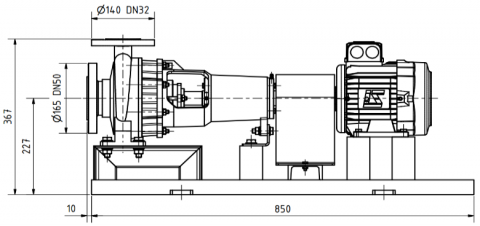
The centrifugal pump of the current study contains one suction and a single discharge canal as well as a circular spiral-shaped volute/casing. The geometry was realized on SolidWorks using [19]. Figure 1 provides a schematic drawing of the pump, and the main characteristics are summarised in Table 1.
Table 1. The main characteristics of the studied centrifugal pump
|
Suction diameter (mm) |
Discharge diameter (mm) |
Inlet pressure (bar) |
Outlet pressure (bar) |
Rpm (tr/min) |
|
60 |
55 |
0.5 |
2 |
720 |
Figure 1. The overall plan of the studied centrifugal pump [19]
This section explains the results of the research and offers a comprehensive discussion. The results are displayed in figures, graphs, tables, and others.
3.1 Impeller design
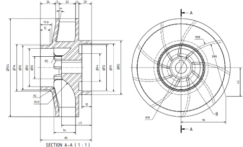
A Centrifugal pump translates rotating energy, usually delivered via a motor, to a moving fluid. The two primary components involved in the energy conversion process are the impeller and the casing. Passing through the impeller, the fluid gains both velocity and pressure [20, 21]. As a result, the impeller itself is a key part of a centrifugal pump, since it acts as the kinetic energy source. The impeller features, which are studied are summarized in Table 2.
Table 2. Impeller main characteristics
|
Outer diameter (mm) |
Inner diameter (mm) |
number of blades |
Tilt angle (deg) |
|
154 |
60 |
8 |
60 |
Figure 2. Impeller detailed plan [9]
The impellers can either be open, semi-open, or closed. As a further point, the impellers could be single or double suction. A single-suction impeller enables liquid to flow into the blade center from a single direction. A double-suction impeller will allow liquid to penetrate to the center of the impeller blades from both directions concurrently [20]. A single-suction closed impeller design will be considered in this study. The pump design was carried out using SolidWorks employing the actual dimensions, which are shown in Figure 2.
3.2 Casing design
The pump casing supplies a pressure limit to the pump and includes channels to correctly steer suction and discharge flow [10]. Furthermore, it decelerates the liquid flow. As per Bernoulli's principle, the volute converts kinetic energy into pressure by reducing the water velocity whilst increasing the pressure. The volute casing reviewed here has been designed per the coil pump's dimensions. The resulting assembly geometry is exhibited in Figure 3.
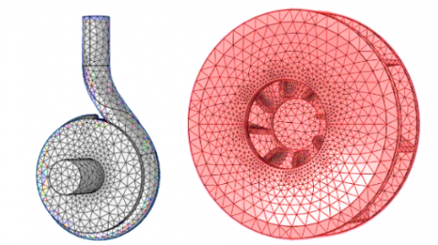
Figure 3. 3D view of the global final geometry
3.3 Mesh structure
A free tetrahedral mesh was applied for the global final geometry. The mesh characteristics are summarized in Table 3 and the final mesh structure is illustrated in Figure 4.
Table 3. Mesh composition
|
Nodes number |
Max element size |
Min element size |
|
88528 |
0.0251 |
0.00183 |
Figure 4. Free tetrahedral mesh of the studied geometry
3.4 Frozen rotor study
The Frozen Rotor study was used to compute the velocity, pressure, and turbulence in Comsol Multiphysics. The frozen rotor approximation implies that the flow in the rotation domain, as stated in the rotation coordinate system, is entirely developed. For that reason, it is generally used in rotating machinery and is viewed as a special case of a Stationary study. The rotating parts are kept frozen in position, and the rotation is accounted for by the inclusion of centrifugal and Coriolis forces. This study is especially suited for the flow in rotating machinery where the topology of the geometry does not change with rotation. It is also utilized to compute the initial conditions for time-dependent simulations of the flow in rotating machinery [22].
3.5 Governing equations
3.5.1 The k-ε turbulence model
The k-ε model is one of the widely used turbulence models for industrial applications. This module includes the standard k-ε model. The model introduces two additional transport equations and two dependent variables: the turbulent kinetic energy, k, and the turbulent dissipation rate, ε. The turbulent viscosity musityisis $\mu_{\mathrm{T}}$ is modeled as [12] Eq. (1):
$f_{\beta}=\frac{1+680 \chi_{k}^{2}}{1+400 \chi_{k}^{2}}, \chi_{k} \leq 0, \chi_{k}>0$
$\chi_{k}=\frac{1}{\omega^{3}}\left(\nabla k_{.} \nabla \omega\right)$
$\mu_{T}=\rho C_{\mu} \frac{k^{2}}{\varepsilon}$ (1)
where, Cμ is a model constant; k the Kinetic energy [J].
The transport equation for k reads:
$\rho \frac{\partial \mathrm{k}}{\partial \mathrm{t}}+\rho \mathrm{u} \cdot \nabla \mathrm{k}=\nabla \cdot\left(\left(\mu+\frac{\mu_{\mathrm{T}}}{\sigma_{\mathrm{k}}}\right) \nabla \mathrm{k}\right)+\mathrm{pk}-\rho \varepsilon$ (2)
where, ρ: The turbulent dissipation rate [m2/s3]; μT: Turbulent viscosity [m2/s]; ε: The molecular, eddy viscosity [Pa.s]; P: The Pressure [Pa]; σk: Experimental model constant; $\nabla k$: Kinetic energy gradient [J].
The production term Pk is:
$P k=\mu_{T}\left(\nabla u:\left(\nabla u+\nabla u^{T}\right)-\frac{2}{3}(\nabla \cdot u) 2\right)-\frac{2}{3} \rho k \nabla \cdot u$ (3)
where, $\nabla u^{\mathrm{T}}$: Turbulent velocity gradient [m/s]; u: x velocity component [m/s].
The transport equation for $\varepsilon$ reads:
$\rho \frac{\partial \varepsilon}{\partial t}+\rho u . \nabla \varepsilon=\nabla .\left(\left(\mu+\frac{\mu_{T}}{\sigma_{\varepsilon}}\right) \nabla \varepsilon\right)+C_{\varepsilon l} \frac{\varepsilon}{k} p_{k}-C_{\varepsilon 2} \rho \frac{\varepsilon^{2}}{k}$ (4)
where, $C_{\varepsilon l}$: model constants.
The model constants in Eq. (1), Eq. (2), and Eq. (4) are determined from the experimental data [1] and the values are listed in Table 4 [22].
Table 4. Model constants
|
Constant |
Value |
|
cμ |
0.09 |
|
cε1 |
1.44 |
|
cε2 |
1.92 |
|
σk |
1.0 |
|
σε |
1.3 |
The constants are: cμ: k-ε Model constant; cε1: Experimental model constant; cε2: Experimental model constant; σk: Dissipation per unit turbulent kinetic energy [m2/s2]; σε: Closure coefficients in turbulence kinetic-energy equation.
3.5.2 The k-ω turbulence model
The k-ω model solves for the turbulent kinetic energy, k, and the dissipation per unit of turbulent kinetic energy, ω. The CFD Module has the Wilcox revised k-ω model [22, 23]:
$\rho \frac{\partial k}{\partial t}+\rho u . \nabla k=p_{k}-\rho \beta^{*} k \omega+\nabla \cdot\left(\left(\mu+\sigma^{*} \mu_{T}\right) \nabla k\right)$ (5)
$\rho \frac{\partial \omega}{\partial t}+\rho u . \nabla \omega=\alpha \frac{\omega}{k} p_{k}-\rho \beta^{*} \omega^{2}+\nabla .\left(\left(\mu+\sigma \mu_{T}\right) \nabla \omega\right)$ (6)
where, α: Model constant; ω: Closure coefficients in the specific dissipation rate equation; β*, σ*: Turbulence-model coefficient; t: Time [s]; $\mu_{\mathrm{T}}=\rho \frac{\mathrm{k}}{\omega} ; \alpha=\frac{13}{25} ; \beta=\beta_{0} f_{\beta} ; \beta^{*}=\beta_{0}^{*} f_{\beta} ; \sigma=\frac{1}{2} ; \sigma^{*}=\frac{1}{2} ; \beta_{0}=\frac{13}{125}$; $f_{\beta}=\frac{1+70 \chi_{\omega}}{1+80 \chi_{\omega}} ; \chi_{\omega}=\left|\frac{\Omega_{i j} \Omega_{j k} \Omega_{k i}}{\left(\beta_{0}^{*} \omega\right)^{3}}\right| ; \beta_{0}^{*}=\frac{9}{100} ; f_{\beta}:$ Round-jet function.
Ωij is the mean rotation-rate tensor:
$\Omega_{i j}=\frac{1}{2}\left(\frac{\partial \overline{\mathrm{u}}_{i}}{\partial \chi_{j}}-\frac{\partial \overline{\mathrm{u}}_{j}}{\partial \chi_{i}}\right)$ (7)
Sij is the mean strain-rate tensor:
$\mathrm{S}_{i j}=\frac{1}{2}\left(\frac{\partial \overline{\mathrm{u}}_{i}}{\partial \chi_{j}}+\frac{\partial \overline{\mathrm{u}}_{j}}{\partial \chi_{i}}\right)$ (8)
Pk is given by Eq. (3). The following auxiliary relations for the dissipation, ε, and the turbulent mixing length, l∗, are also used:
$\varepsilon=\beta^{*} \omega \mathrm{k} ; l_{\text {mix }}=\frac{\sqrt{k}}{\omega}$ (9)
3.5.3 The k-ω SST turbulence model
To combine the superior behavior of the k-ω model in the near-wall region with the robustness of the k-ε model, Menter [24] introduced the SST (Shear Stress Transport) model which interpolates between the two models. The version of the SST model in the CFD module includes a few well-tested [25] modifications, such as production limiters for both k and ω, the use of S instead of Ω in the limiter for μT and a sharper cut-off for the cross-diffusion term. It is also a low Reynolds number model. In other terms, it does not apply wall functions. The Low Reynolds number refers to the region, which is close to the wall where viscous effects dominate. The model equations are formulated in terms k and ω, [22]:
$\rho \frac{\partial k}{\partial t}+\rho$ u. $\nabla k=p-\rho \beta_{0}^{*} k \omega+\nabla \cdot\left(\left(\mu+\sigma_{k} \mu_{T}\right) \nabla k\right)$
$\rho \frac{\partial \omega}{\partial \mathrm{t}}+\rho u . \nabla \omega=\frac{\rho \gamma}{\mu_{\mathrm{T}}} \mathrm{p}-\rho \beta \omega^{2}+\nabla \cdot\left(\left(\mu+\sigma_{\omega} \mu_{\mathrm{T}}\right) \nabla \omega\right)+2(1-\left.\mathrm{f}_{\mathrm{v} 1}\right) \frac{\rho \sigma_{\omega 2}}{\omega} \nabla \omega . \nabla \mathrm{k}$ (10)
where,
$P=\min \left(P_{k}, 10 \rho \beta_{0}^{*} k \omega\right)$ (11)
And Pk is given in Eq. (3). The turbulent viscosity is given by:
$\mu_{\mathrm{T}}=\frac{\rho a_{1}}{\max \left(a_{1} \omega, S f_{v_{2}}\right)}$ (12)
where, fv1 and fv2 are the auxiliary function in turbulence model, fv1 is equal to zero away from the surface (k-ε model), and switches over to one inside the boundary layer (k-ω model) [23]. This reflects the efficiency of combining the two models, S is the characteristic magnitude of the mean velocity gradients, a1: model canstant (0, 31).
$\mathrm{S}=\sqrt{2 \mathrm{~S}_{i j} \mathrm{~S}_{i j}}$ (13)
The model constants are defined through interpolation of appropriate inner and outer values:
$\phi=f_{v 1} \phi_{1}+\left(1-f_{v 1}\right) \phi_{2}$ for $\phi=\beta, \gamma, \sigma_{k}, \sigma_{\omega}$ (14)
where, the constants $\varphi$ of the model are calculated from the constants $\varphi 1$ and $\varphi 2 ; \gamma$ : Momentum thickness [m].
The interpolation functions fv1 and fv2 are defined as:
$f_{v 1}=\tanh \left(\theta_{1}^{4}\right)$
$\theta_{1}=\min \left[\max \left(\frac{\sqrt{k}}{\beta_{0}^{*} \omega l_{w}}, \frac{500 \mu}{\rho \omega l_{w}^{2}}\right), \frac{4 \rho \mu \sigma_{\omega 2} k}{C D_{\mathrm{k} \omega} l_{w}^{2}}\right]$ (15)
where,
$C D_{\mathrm{k} \omega}=\max \left(\frac{2 \rho \sigma_{\omega 2}}{\omega} \nabla \omega . \nabla \mathrm{k}, 10^{-10}\right)$ (16)
where, lw is the distance to the closest wall, and CDkω positive portion of the cross-diffusion in ω-transport equation.
4.1 Grid sensitivity
The convergence plays an essential role in obtaining accurate results through numerical means as finite element analysis. As a consequence, the sensitivity analysis needs to be performed on the studied turbulence models, which allow to determine the optimal model, to reduce dissipation errors in terms of accuracy and computational cost. In this regard, the impact of the mesh quality (dimension, total number of elements, error) on the simulation results was studied in the three turbulence models using a free tetrahedral mesh with different dimensions: i) coarser, ii) normal and iii) fine.
A detailed comparison is indicated in the Table 5. This study allowed us to determine both the optimal mesh type for a CFD analysis, the least expensive turbulence model and to confirm the accuracy of the results. The convergence evolution of the three studied turbulence models a) K-Ω, b) K-Ω SST & c) $\mathrm{K}-\varepsilon$ is depicted in Figure 5.
On the one hand, the best calculation precision and the lowest error, (8.13×10⁻⁷), achieved using the k-ω model. While the k-ε model provided an error of 8.92×10⁻⁶, the k-ω SST model could only achieve 2.14×10⁻⁵. In addition, the convergence of the latter was accomplished in just 18min 16s, and the $\mathrm{k}-\varepsilon$ model required 58min 50s. More importantly, the k-ω model exceeded 1 hour (results were obtained using an intel® Core (Tm) i5-7500 CPU).
a) K-Ω
b) K-Ω SST
c) K-Ε
Figure 5. Convergence evolution of the three studied turbulence models
Table 5. Analysis of mesh sensitivity in the three turbulences models
|
Models |
Numbers of elements |
Edge element |
Average element quality |
Max pressure (bar) |
Max Velocity magnitude (m/s) |
Iteration number |
Error |
CPU time |
|
K-Ε |
111857 |
2202 |
0,645 |
1,5452 |
9,127 |
371 |
4,35×10⁻⁶ |
37min 17s |
|
139649 |
2214 |
0,653 |
1,5569 |
9,443 |
378 |
3,06×10⁻⁶ |
53min 24s |
|
|
158737 |
2323 |
0,657 |
1,5790 |
9,564 |
389 |
8,92×10⁻⁶ |
58min 50s |
|
|
K-Ω |
111857 |
2202 |
0,645 |
1,8340 |
10,164 |
387 |
3,44×10⁻⁷ |
46 min 45s |
|
139649 |
2214 |
0,653 |
1,8244 |
10,301 |
405 |
8,13×10⁻⁷ |
1h 2min 24s |
|
|
158737 |
2323 |
0,657 |
1,8425 |
10,403 |
404 |
3,29×10⁻⁷ |
1h 7min 23s |
|
|
K-ΩSST |
11560 |
848 |
0,562 |
1,5952 |
8,1988 |
234 |
1,36×10⁻⁷ |
3 min 49s |
|
38045 |
1350 |
0,630 |
1,8120 |
9,7911 |
281 |
2,56×10⁻⁶ |
9min 34s |
|
|
70163 |
1735 |
0,651 |
1,8532 |
10,072 |
312 |
2,14×10⁻⁵ |
18min 16s |
4.2 Velocity distribution
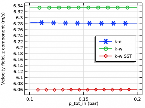
Water velocity evolution as a function of inlet pressure is illustrated in Figure 6. The effect of increasing inlet pressure on velocity was not noticed owing to the significant variance between the three models' velocity distributions; also, on account of the slight pressure increase.
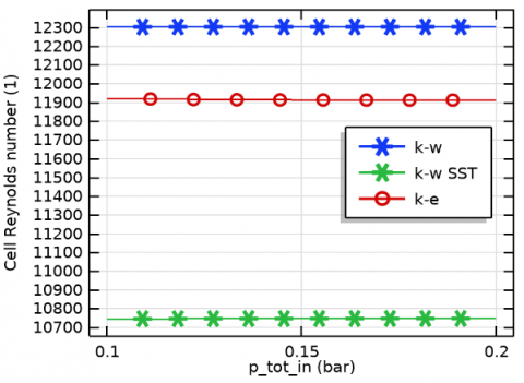
As is revealed in Figure 6, the k-ω model provided the highest discharge velocity compared to the other two models. This behavior would justify the higher Reynolds number across the discharge section in this turbulence model (Figure 7).
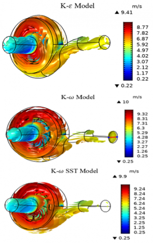
Figure 8 affirms that all the three studied models present a fair degree of similarity. However, the maximum velocity was generated by the k-ω sst model, which exceeded 9.5 m/s. This same model obtained the lowest outlet velocity (Figure 6).
According to Bernoulli's principle, the volute converts kinetic energy into pressure by reducing velocity while increasing pressure. For that reason, the maximum average water velocity was generated by the k-ω SST model (Figure 7).
Figure 6. Maximum water velocity evolution as a function of inlet pressure
Figure 7. Reynolds number evolution in the discharge section for the three studied models
Figure 8. Average water velocity distribution in the volute for the three studied models $\mathrm{K}-\varepsilon$, K-Ω, & K-Ω SST
4.3 Pressure distribution
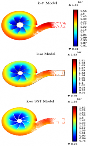
Figure 9 depicts a close-up of the water pressure profiles in the rotational zone, for the three considered models. The highest-pressure contour was obtained by the k-ω SST model. Indeed, maximum pressure of 1,85 bar was reached with an average pressure of 1,16 bar. This makes perfect sense since this model provided the highest water velocity distribution in the volute. This high velocity has been was converted into dynamic pressure. Consequently, the highest outlet pressure was recorded for this model (Figure 10). As for the influence of increasing inlet pressure on the outlet pressure, it is not visible due to the large difference between the pressure distributions of the three models.
Figure 9. Water pressure [bar] contours in the volute for the three considered models a) K-Ω, b) K-Ω SST & c) $\mathrm{K}-\varepsilon$
Figure 10. Maximum outlet pressure as a function of inlet pressure
The static pressure profiles, in the impeller domain, are depicted in Figure 11, the highest static pressure was generated by the k-w SST model (1.36 bar) as it provided the maximum water pressure and velocity in the volute (Figure 6, Figure 11).
Figure 11. Static pressure contour in the impeller domain
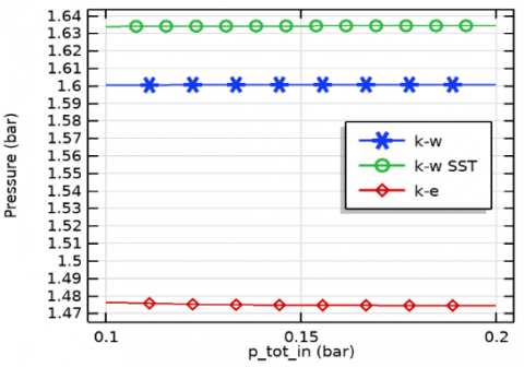
Figure 12. Pump performance curve for the three studied cases
The pump's performance curve is presented in Figure 12. The total pressure at the inlet is expressed in terms of the pressure head, H, which is equal to [22]:
$H=\frac{\Delta p_{t o t}}{\rho g}$ (16)
where, ∆ptot: pressure difference [bar], g: standard acceleration of gravity [m/s2].
The highest head (10.85 m) was achieved by the k-ω SST model and generated the greatest outlet pressure. As a result, a better water height was recorded.
The main aim of this research was to investigate how three numerical turbulence models could affect both the convergence and the performance of the flow simulation through a comparative computational analysis, which is based on COMSOL Multiphysics, in which the flow modeling process was based mostly upon stationary Navier-Stokes equations. equally, the impact of these models on the numerical CFD simulation was also taken into account.
The analyzed findings allowed us to conclude that the best computational accuracy is obtained by the k-ω model, whereas the lowest was given by the $k-\omega$ SST model. Nevertheless, a significantly low calculation cost was attained through the latter. Likewise, a better pumping performance was also recorded. The collected data of this investigation also evinced the computation under $k-\omega$ SST was successfully able to achieve convergence after only 312 iterations. However, the $k-\omega$ model and the $\mathrm{k}-\varepsilon$ model provided more accuracy at the expense of the computational cost and the memory used.
The proposed study can be implemented in centrifugal pump modeling and design. It is also applicable in:
- Research, which is industrially implemented for centrifugal pump design optimization;
- Further experiments involving COMSOL Multiphysics software for enhancing centrifugal pump efficiencies.
The authors would like to thank ESTI Annaba LTSE laboratory members for their great help. work: We would also like to express our sincere thanks to LR3MI laboratory for allowing us to use their COMSOL Multiphysics software license. This work was supported by the Algerian Ministry of Higher Education & Scientific Research, PRFU Research Project: Contribution to the study of modeling and simulation of the energy and matter transfer in laminar and turbulent flows. Project Code A11N01EP230220220002 (2022).
|
cμ |
k-ε Model constant |
|
cε1 |
Experimental model constant |
|
cε2 |
Experimental model constant |
|
CDkω |
Positive portion of the cross-diffusion in ω-transport equation |
|
fβ |
Round-jet function |
|
fv1, fv2 |
Auxiliary function in turbulence model |
|
H |
Water head [m] |
|
lw |
Distance to the closest wall [m] |
|
lmix |
Turbulent mixing length |
|
K |
Kinetic energy [J] |
|
P |
Pressure [Pa] |
|
pk |
Production term |
|
S |
Characteristic magnitude of the mean velocity gradients |
|
Sij |
Mean strain-rate tensor |
|
t |
Time [s] |
|
U |
x velocity component [m/s] |
|
Greek symbols |
|
|
μT |
Turbulent viscosity [m2/s] |
|
ρ |
Turbulent dissipation rate [m2/s3] |
|
ε |
Molecular, eddy viscosity [Pa.s] |
|
μ, μT |
Dissipation per unit turbulent kinetic energy [m2/s2] |
|
σk |
Dissipation per unit turbulent kinetic energy [m2/s2] |
|
σε |
Closure coefficients in turbulence kinetic- energy equation |
|
ω |
Closure coefficients in the specific dissipation rate equation |
|
β*, σ* |
Turbulence-model coefficient |
|
α, β, σ |
Model constant |
|
γ |
Momentum thickness [m] |
|
ϕ |
Absolute value of χp |
|
θ |
Pope’s nondimensional measure of vortex stretching parameter |
|
χω |
Rotation tensor |
|
χp |
Closure coefficients in turbulence kinetic- energy equation |
[1] Wilson, K.C., Addie, G.R., Sellgren, A., Clift, R. (1992). Slurry Transport Using Centrifugal Pumps. Elsevier Science Publishers Ltd., Essex, England.
[2] Mostefa, B., Kaddour, R., Embarek, D., Amar, K. (2021). Analysis and optimization of the performances of the centrifugal compressor using the CFD. International Journal of Heat and Technology, 39(1): 107-120. https://doi.org/10.18280/ijht.390111
[3] Hedi, L., Hatem, K., Ridha, Z. (2010). Numerical flow simulation in a centrifugal pump. International Renewable Energy Congress, pp. 300-304.
[4] Mentzos, M., Filios, A., Margaris, P., Papanikas, D. (2004). A numerical simulation of the impeller-volute interaction in a centrifugal pump. Proceedings of International Conference from Scientific Computing to Computational Engineering, Athens, pp. 1-7.
[5] Shah, S.R., Jain, S.V., Patel, R.N., Lakhera, V.J. (2013). CFD for centrifugal pumps: A review of the state-of-the-art. Procedia Engineering, 51: 715-720. https://doi.org/10.1016/j.proeng.2013.01.102
[6] Bacharoudis, E.C., Filios, A.E., Mentzos, M.D., Margaris, D.P. (2008). Parametric study of a centrifugal pump impeller by varying the outlet blade angle. The Open Mechanical Engineering Journal, 2(1): 75-83. http://dx.doi.org/10.2174/1874155X00802010075
[7] Anagnostopoulos, J.S. (2006). CFD analysis and design effects in a radial pump impeller. WSEAS Transactions on Fluid Mechanics, 1(7): 763.
[8] Patel, K., Ramakrishnan, N. (2006). CFD analysis of mixed flow pump. In International ANSYS Conference Proceedings.
[9] Pope, S. (2000). Turbulent Flows. Cambridge: Cambridge University Press. http://dx.doi.org/10.1017/CBO9780511840531
[10] Wilcox, D.C. (1993). Turbulence Modeling for CFD. California: DCW industries Inc.
[11] Wilcox, D. (1991). A half century historical review of the k-omega model. In 29th Aerospace Sciences Meeting, p. 615. https://doi.org/10.2514/6.1991-615
[12] El-Behery, S.M., Hamed, M.H. (2011). A comparative study of turbulence models performance for separating flow in a planar asymmetric diffuser. Computers & Fluids, 44(1): 248-257. https://doi.org/10.1016/j.compfluid.2011.01.009
[13] Gorji, S., Seddighi, M., Ariyaratne, C., Vardy, A.E., O’Donoghue, T., Pokrajac, D., He, S. (2014). A comparative study of turbulence models in a transient channel flow. Computers & Fluids, 89: 111-123. https://doi.org/10.1016/j.compfluid.2013.10.037
[14] Liu, H.L., Liu, M.M., Dong, L., Ren, Y., Du, H. (2012). Effects of computational grids and turbulence models on numerical simulation of centrifugal pump with CFD. In IOP Conference Series: Earth and Environmental Science, 15(6): 062005. https://doi.org/10.1088/1755-1315/15/6/062005
[15] Menter, F.R. (1992). Performance of popular turbulence model for attached and separated adverse pressure gradient flows. AIAA Journal, 30(8): 2066-2072. https://doi.org/10.2514/3.11180
[16] Bulat, M.P., Bulat, P.V. (2013). Comparison of turbulence models in the calculation of supersonic separated flows. World Applied Sciences Journal, 27(10): 1263-1266. https://doi.org/10.5829/idosi.wasj.2013.27.10.13715
[17] Selim, S.M., Hosien, M.A., El-Behery, S.M., Elsherbiny, M. (2016). Numerical analysis of turbulent flow in centrifugal pump. In Proceedings of the 17th Int. AMME Conference, pp. 21. https://doi.org/10.21608/amme.2016.35279
[18] Hundshagen, M., Casimir, N., Pesch, A., Falsafi, S., Skoda, R. (2020). Assessment of scale-adaptive turbulence models for volute-type centrifugal pumps at part load operation. International Journal of Heat and Fluid Flow, 85: 108621. https://doi.org/10.1016/j.ijheatfluidflow.2020.108621
[19] Alves, P. Free CAD Designs, Files & 3D Models | The GrabCAD Community Library. https://grabcad.com/library/centrifugal-pump-71/details?folder_id=5639539, accessed on Mar. 23, 2022.
[20] U.S. Department of Energy, Doe Fundamentals Handbook - Mechanical Science (Volume 1 Of 2). 2016. http://energy.gov/sites/prod/files/2013/06/f2/h1018v2.pdf.
[21] Myaing, K., Win, H.H. (2014). Design and analysis of impeller for centrifugal blower using solid works. International Journal of Scientific Engineering and Technology Research, 3(10): 2138-2142.
[22] https://www.comsol.com/, accessed on Sept. 2, 2021.
[23] Al-Obaidi, A.R. (2019). Effects of different turbulence models on three-dimensional unsteady cavitating flows in the centrifugal pump and performance prediction. International Journal of Nonlinear Sciences and Numerical Simulation, 20(3-4): 487-509. https://doi.org/10.1515/ijnsns-2018-0336
[24] Menter, F.R. (1994). Two-equation eddy-viscosity turbulence models for engineering applications. AIAA Journal, 32(8): 1598-1605. https://doi.org/10.2514/3.12149
[25] Menter, F.R., Kuntz, M., Langtry, R. (2003). Ten years of industrial experience with the SST turbulence model. Turbulence, Heat and Mass Transfer, 4(1): 625-632.