Ameur Kada* | Mohammed Elmir | Abderrahim Mokhefi | Mohamed Bouanini | Pierre Spiteri
© 2022 IIETA. This article is published by IIETA and is licensed under the CC BY 4.0 license (http://creativecommons.org/licenses/by/4.0/).
OPEN ACCESS
In this paper, the behavior of an elastic barrier subjected to isothermal laminar flow of Al2O3-water nanofluid in a channel has been studied numerically by the finite element method. A CFD based on the arbitrary Lagrange-Euler (ALE) formulation, has been developed in an attempt to solve the Navier-Stokes and stress-strain equations of the structure. The objective is to study the effects of inertia (Re) and nanoparticle volume fraction (φ) on the overall hydrodynamic behavior, as well as on the nanofluid-structure interface. The results showed that the deformation of the structure was mainly caused by the pressure loading of the nanofluid and the viscous drag imposed on the structure walls. In addition, the structure was strongly affected by the increase in Reynolds number and volume fraction of the nanoparticles. Finally, a numerical correlation was established to determine the maximum displacement caused by the bending of the structure.
nanofluid-structure interaction, finite element method, Navier-stokes, arbitrary Lagrange-Euler, (ALE)
The industrial field is hardly devoid of the fluid-structure interaction phenomena particularly between fluids and baffles inside pipelines. Heat exchangers, for instance, contain such baffles to limit the fluid movement for cooling or heating purposes. In the context of heat transfer, nanofluid are of high interest due to their ability to improve the performance of exchangers. However, introducing nanoparticles modifies the physical properties of the nanofluid, to which investigating their effect on solid structures becomes necessary. On the other hand, the fluid flow imposes forces on the boundaries of the structure, which forces it to displace. This movement will in turn influence the conditions of the flow. Solid structures are generally in contact with at least one fluid. Therefore, the fluid and solid movements are not independent, but are coupled by a number of kinematic and dynamic conditions. The fluid and the structure, considered as a whole, thus behave as a coupled dynamic system.
The fluid-structure interaction field is a growing research subject, to which the addressed problems are very frequent in industrial applications involving two concurrent sub-fields, a fluid and a structure. Mehryan et al. [1] numerically studied the hydrodynamic and thermal performance of a Newtonian fluid in the computational domain of the L-shaped cavity, including the flexible baffle. Presented the formulation of the equations in the arbitrary Lagrangian-Eulerian (ALE) coordinate system the study of the motion of a fluid within a solid poses numerous key question in fluid mechanics.
Later, in the sixties of the last century. Ghalambaz et al. [2] has given a numerical study of a fluid-structure interaction representing an elastic oscillating fin fixed to the hot vertical wall of a square cavity. Shahabadi et al. [3] have studied the flow of a non-Newtonian fluid and the heat transfer in a cavity with an elastic flexible fin fixed to the hot wall of the cavity. They examined the solid-fluid interaction (FSI). The Arbitrary Lagrangian-Eulerian method is used to describe the fluid motion with the elastic wall in the fluid-structure interaction model. Nithyadev et al. [4] using the finite volume method. They investigated the effects of the aspect ratio of the cavity and different relative positions. Berry and Reissner [5] studied the behavior of a cylindrical shell filled with pressurized fluid. Coale and Nagano [6], on the other hand, calculated the axisymmetric modes of a cylindrical shell, joined to a hemispherical shell, both filled with liquid.
Later, Paidoussis et al. [7] presented a comprehensive study on the dynamics and stability of structures subjected to a fluid flow. Paidoussis and Li [8] then studied the dynamics of pipes transporting fluid and presented a selective assessment of the research undertaken. Lindholm et al. [9] was then the first to experimentally calculate the resonance frequencies of cantilever plates totally or partially immersed in water. This was also compared against theoretical results, making it possible to better assess the influence of the flow on the structure.
Later, Lakis and Paidoussis [10] developed a circumferential hybrid finite element model, based on the classical shell theory, to analyze the dynamic behavior of a vertical cylindrical reservoir partially filled with liquid. Lindholm et al. [11] was another pioneer to investigate vibrations of cylindrical shells partially filled with liquid. On the other hand, Mittal and Tezduyar [12] studied the variation of the acoustic velocity as a function of the ratio between tubes’ thickness and radius, i.e. closing a valve to increase the pressure inside pipes, which caused waves to propagate along the channel. Meanwhile, Messahl et al [13] numerically investigated the industrial problem of a fluid-structure interaction and cavitation in a single-bend pipe system. Later, Raoul et al. [14] examined the solid-fluid coupling, via numerical modelling, for a thin body solid. In this case, the flow was described by the Navier-Stokes equations, the deformation of the body followed the Neo-Hooke a model, and the coupling between the fluid and the structure was implemented via Lagrange multipliers.
Goura et al. [15] then formulated an interpolation technique for displacement data between fluidic and structural numerical simulation meshes. On the other hand, Tijsseling and Lavooij [16] explored the interaction between water hammers and pipe movements. Meanwhile, Jhung et al. [17] investigated the reliability of fluid filled tanks on the modal characteristics, taking into account fluid-structure interaction effects. They utilized the finite element method for the structure, while making use of the method of mass added to the structure to simplify the problem. This allowed them to obtain the displacement and natural frequency of filling the tank, showing that the added mass resulted with higher frequencies. Furthermore, Lin et al. [18] was successful in numerically simulating the flow through a micro channel equipped with an elastic membrane. This allowed them to study the effects of various parameters, mainly the elasticity of the membrane, the viscosity of the liquid, and the geometry of the elastic membrane, on the displacement of the membrane tip, its maximum shear stress, and it is bending moment. Later, Sigrist et al. [19] conducted a modal analysis of an industrial structure coupled with a fluid via numerical techniques of fluid-structure couple of calculations. The nature of the structure was ax symmetric in geometry, where by the modeling of the problem was carried out using an ax symmetric finite elements approach implemented using Fourier series discretization in finite elements. On the other hand, Liu et al. [20] studied, through numerical simulations, the interaction between a fluid and a flexible structure using Navier-Stokes and Euler-Bernoulli equations. In this study, both laminar and turbulent flows were investigated. In another study, Grandmont and Maday [21] studied, via mathematical and numerical analyses, the phenomena of interaction between a fluid and a mobile solid, rigid and deformable structures. Later, De Ridder et al. [22] presented a study on the vibratory behavior of a flexible cylinder subjected to axial flow.
In addition, Lin and Tsai [23] then presented a finite element study to analyze the nonlinear vibrations of fluid transport pipes using Timoshenko theory. Their model consisted of three degrees of freedom, nodal, beam elements, whereby the expressions of kinetic energy and deformations of the structure and fluid were used to determine rigidity, mass, and damping matrices of the problem. Their results elaborated on the influence of flow induced vibrations on the natural frequencies of the structure. On the other hand, Stein and Tobriner [24] presented a numerical solution to the equation of motion which describes the behavior of an elastic-supported pipe of infinite length carrying an ideal pressurized fluid. This allowed them to interpret the effects produced due to internal pressure forces and mass and damping matrices, as well as to evaluate the influence of flow induced vibrations on the natural frequencies of the structure later Kohli and Nakra [25] conducted a dynamic stability analysis of a fluid-filled stepped pipe using the Euler-Bernoulli theory, implemented in finite elements, whereby eigen frequencies were compared with respect to a pipe section.
A similar work was conducted by Aldraihem [26], in which the dynamic stability of a fluid in a rigid collared pipe was examined using the Euler-Bernoulli beam theory, via the finite element tool, to predict the dynamic stability of the pipe. Meanwhile, Chadi et al. [27] studied heat exchangers, with different mini channels geometry sections, using three different nanoparticles. The results obtained showed that the increase in the surface area between the walls of the mini channels and the cooling fluid increases the exchange coefficient, along an increase in Reynolds number. Later, Koribi et al. [28] presented a numerical study on flow characteristics and thermal fields surrounding a rotating cylinder, subjected to small Reynolds numbers Lastly, Srinivasa et al. [29] investigated the fluid-structure interaction resulting from the sole effects of the flow of water on the deformation of the structure.
Sabbar et al. [30] studied unsteady mixed convection in a cavity-channel ensemble. They solved the governing equations for the interaction between the fluid and the elastic wall, the effects of elastic modulus, buoyancy/viscosity ratio and inertia/viscosity ratio. They showed that the presence of the elastic walls improves the heat transfer compared to the rigid cavity walls.
To come now to the main subject of this article, the obstacles implanted in a channel are subjected not only to the base fluid (water), but also to the nanoparticles carried by the base fluid (nanofluid). To the authors' knowledge and according to the existing literature, the behavior of a structure subjected to the flow of a nanofluid has not yet been studied. The objective of this research was therefore to study, in fluid dynamics, the effects of the Reynolds number and the volume fraction of the nanoparticles, present in the base fluid, on the flow.
Thus, the objective of this paper is to study the behavior of the elastic structure and the flow and their interaction in the channel, we have conducted a thorough investigation to find out if the FSI is used in such a setup. From the results of the investigation, we found that this problem has not been studied yet. In the future, the study can be extended for higher Reynolds numbers, different position of obstacle; different types of nanofluid.
A schematic of the physics of the problem is shown in Figure 1. A horizontal flow channel, in the middle of which there exists an obstacle, a narrow vertical structure, is considered. The nanofluid flows from left to right, unless the obstacle forces it into a narrower passage in the upper part of the channel and places a force on the walls of the structure resulting from the viscous drag and pressure of the fluid. As the obstacle is made of a deformable material, it bends under the applied load. The thermophysical proprieties of water and Alumina are given in Table 1.
In this work, a single-phase model, which considers the nanofluid as a continuous medium, is used. Assuming that the nanoparticles are well dispersed in the base fluid, the properties of the nanofluid can therefore be calculated according to the following formulas:
The effective density of the nanofluid is calculated by:
${{\rho }_{nf}}=\varphi {{\rho }_{p}}+\left( 1-\varphi \right){{\rho }_{f}}$ (1)
The effective dynamic viscosity of the nanofluid is given by Brinkman relation as follows:
${{\mu }_{nf}}={{\mu }_{f}}{{\left( 1-\varphi \right)}^{-2.5}}$ (2)
where, μf is the dynamic viscosity of the water.
Figure 1. Flexible structure subjected to a horizontal flow
Table 1. Physical properties of the base fluid and the nanoparticles
|
Physical thermo property |
Base fluid (water) |
Alumina (Al2O3) |
|
$\mu$ (Ns/m2) |
8.55 × 10⁻⁴ |
|
|
$\rho$ (kg/m3) |
997.1 |
3970 |
|
$C_{p}$ (J/kg k) |
4179 |
765 |
|
k (w/m k) |
0.613 |
40 |
|
α (m2 /s) |
1.47 × 10⁷ |
1.32 × 10⁻⁵ |
|
β (K−1) |
21 × 10−5 |
0.85 × 10⁻⁵ |
2.1 Constitutive model simplifications
To simplify the considered problem, the following assumptions are made:
The dimensional equations governing this flow, in Cartesian coordinates, thus become:
$\frac{\partial u}{\partial x}+\frac{\partial v}{\partial y}=0$ (3)
${{\rho }_{\text{nf}}}\left( \frac{\partial u}{\partial t}+u\frac{\partial u}{\partial x}+v\frac{\partial u}{\partial y} \right)=-\frac{\partial p}{\partial x}+{{\mu }_{\text{nf}}}\left( \frac{{{\partial }^{2}}u}{\partial {{x}^{2}}}+\frac{{{\partial }^{2}}u}{\partial {{y}^{2}}} \right)$ (4)
${{\rho }_{\text{nf}}}\left( \frac{\partial v}{\partial t}+u\frac{\partial v}{\partial x}+v\frac{\partial v}{\partial y} \right)=-\frac{\partial p}{\partial x}+{{\mu }_{\text{nf}}}\left( \frac{{{\partial }^{2}}v}{\partial {{x}^{2}}}+\frac{{{\partial }^{2}}v}{\partial {{y}^{2}}} \right)$ (5)
The structural domain is governed by nonlinear elasto-hydrodynamics behavior as follow:
${{\rho }_{S}}\frac{{{\partial }^{2}}{{d}_{S}}}{\partial {{\tau }^{2}}}-\nabla \sigma ={{F}_{v}}$ (6)
the elastic deformation of the fin, resulting from the fluid and pressure forces can be expressed in terms of the Kirchhoff stress tensor as:
$\tau =J{{\sigma }_{s}}$ (7)
$\tau =J{{\sigma }_{s}}$ (8)
where, $F=\left(1+\nabla^{\sigma_{s}}\right), j=\operatorname{det}(\mathrm{f})$, s is the second piola-kirchhoff stress tensor. consider the following dimensionless parameters:
$\tau=\frac{t U}{H}, X^{*} ; Y^{*}=\frac{x ; y}{H}, U^{*} V^{*}=\frac{u ; v}{U}, P^{*}=\frac{p}{\rho_{n f \quad}U^{2}}, d_{s}^{*}=\frac{d_{s}}{H}$ et$\sigma^{*}=\frac{\sigma}{E}$ (9)
The dimensionless behavior of Eqns. (3) to (6) can be formulated as:
$\frac{\partial {{U}^{*}}}{\partial {{X}^{*}}}+\frac{\partial {{V}^{*}}}{\partial {{Y}^{*}}}=0$ (10)
$\frac{\partial U^{*}}{\partial \tau}+U^{*} \frac{\partial U^{*}}{\partial X^{*}}+V^{*} \frac{\partial U^{*}}{\partial Y^{*}}=-\frac{\partial P^{*}}{\partial X^{*}}+\frac{\rho_{\mathrm{f}}}{\rho_{\mathrm{nf}}} \frac{\mu_{\mathrm{nf}}}{\mu_{\mathrm{f}}} \frac{1}{\operatorname{Re}}\left(\frac{\partial^{2} U^{*}}{\partial X^{* 2}}+\frac{\partial^{2} U^{*}}{\partial Y^{* 2}}\right)$ (11)
$\frac{\partial V^{*}}{\partial \tau}+U^{*} \frac{\partial V^{*}}{\partial X^{*}}+V^{*} \frac{\partial V^{*}}{\partial Y^{*}}=-\frac{\partial P^{*}}{\partial Y^{*}}+\frac{\rho_{\mathrm{f}}}{\rho_{\mathrm{nf}}} \frac{\mu_{\mathrm{nf}}}{\mu_{\mathrm{f}}} \frac{1}{\operatorname{Re}}\left(\frac{\partial^{2} V^{*}}{\partial X^{* 2}}+\frac{\partial^{2} V^{*}}{\partial Y^{* 2}}\right)$ (12)
The structural bahavior for the elastic fin is described by the following equation
$\frac{Ca}{{{\rho }_{r}}}\frac{{{\partial }^{2}}d_{s}^{*}}{\partial {{\tau }^{2}}}-\nabla \sigma _{s}^{*}=0$ (13)
where, Re, Ca and ρr are respectively the Reynold number, the Cauchy number and the relative density between the base fluid and the solid fin. They are defined by:
$\operatorname{Re}=\frac{{{\rho }_{\text{f}}}LU}{{{\mu }_{\text{f}}}}$, $Ca=\frac{{{\rho }_{f}}{{U}^{*2}}}{E}$and ${{\rho }_{r}}=\frac{{{\rho }_{s}}}{{{\rho }_{f}}}$ (14)
Notations appearing in Eqns. (1)-(12) are: V =(u, v) are the velocity vectors of fluid and the moving coordinate system, $P^{*}$ is the dimensionless fluid pressure, Fvis the body force acting on the fin (it is taken zero in this study),ds is the fin displacement vector, ρs is the density of solid structure ρf is the water density, ρp is the nanoparticles density and σ is the stress tensor.
Initial-boundary conditions
The initial conditions at τ = 0 are: $U^{*}=V^{*}=0$ and $U_{S}{ }^{*}=0$. The dimensionless boundary conditions are grouped together in Table 2.
Table 2. Boundary conditions
|
Inlet |
structure |
High and low walls |
Outlet |
|
${{U}^{*}}$= 1 ${{V}^{*}}$ = 0 |
${{U}^{*}}$ = ∂τ${{U}_{S}}^{*}$ |
${{U}^{*}}$=${{V}^{*}}$ = 0, ${{U}_{S}}^{*}$ = 0 |
${{P}^{*}}$= 0 |
The system of equations governing the nanofluid flow and the behavior of the structure was solved via the finite element method. A dynamic and triangular mesh, refined at the level of the walls of the structure, was adopted by Figure 3. A convergence criterion where the relative error is strictly less than 10-6 was adopted. A mesh sensitivity analysis was conducted, as illustrated by Figure 2, with respect to the nanofluid velocity measured at the midline of the channel. Table 3 shows the results of this test an optimal mesh of 25704 elements and 526 boundaries showed to be accurate to obtain the appropriate numerical tolerance.
Figure 2. Velocity profile for different meshes
Figure 3. Dynamic mesh of the area of interest, at the level of the obstacle
Table 3. Mesh dependance
|
Element number |
Maximum velocity |
Max displacement |
|
2531 |
1.47309 |
0.0812759 |
|
3248 |
1.49661 |
0.0825469 |
|
7443 |
1.50150 |
0.0831062 |
|
25704 |
1.50282 |
0.0831262 |
|
56643 |
1.50229 |
0.0831276 |
In efforts of validating the model, the obtained results were then compared against the study of Srinivaza Rao et al. [29], as shown in Figure 4.
Figure 4. Validation of the current model against Srinivaza Rao et al. [29]
In this section, the results obtained from the numerical simulation of the hydrodynamic phenomenon as well as the behavior of a stainless-steel structure during the flow of a nanofluid (alumina-water) inside a pipe are presented. The effect of certain control parameters, mainly the Reynolds number (1 < Re <7) and the nanoparticles volume fraction (0 <φ<10%), is highlighted. Results presented include the velocity field, streamlines, pressure distribution, and maximum displacement. It is noted that the flow of the nanofluid was unsteady; however, results were collected at a fixed dimensionless instant, τ = 1332, corresponding to a state of stability.
4.1 Streamlines and velocity
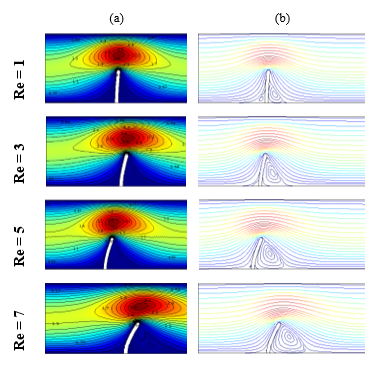
Among the most critical parameters when analyzing hydrodynamic results is the Reynolds number. This number describes the relationship between inertial and viscous. In this study, the procedure to change the Reynolds number (Re) is associated with a change in inertial forces, particularly, via an increase in the rate of entry of the nanofluid to the pipeline. Figure 5 presents the velocity field (a) and streamlines (b) distribution, for different Reynolds numbers (Re = 1, 3, 5 and 7), an alumina nanoparticles volume fraction of φ = 4%, and when the system is close to its stationary state at the dimensionless instant τ>1332.
In general, the flow of the nanofluid in the pipe caused the structure to deform by bending in the direction of the flow. This deformation was due to the viscous drag and pressure loads imposed by the fluid on the structure. On one hand, as the Reynolds number increased, the laminar flow of the nanofluid prompted the structure to deform with a large degree of tilt. On the other hand, there was a considerable increase in flow intensity in the narrow area of the channel above the structure, with an enlargement of the vortex zone produced downstream of the structure. It is noted that, for low Reynolds numbers (Re = 1 in this case), the vortex zones occur upstream and downstream of the structure, where their intensity is greater in the downstream side.
Figure 5. (a) Velocity and (b) Streamline profiles for different Re at φ = 0.04
This latter finding indicates that, although the structure presents an obstacle to the flow of the nanofluid, its flexural deformation under inertial loads gives a certain fluidity in the movement f the fluid downstream.
The existence of alumina nanoparticles suspended in water contributes to a relative increase in the viscosity of the nanofluid when compared with that of the base fluid. This increase in viscosity, as described by Brinkmann's law, leads to an increase in impact forces resulting from the laminar flow viscous drag. Figure 6 shows the effect of changing the volume fraction of the nanofluid (the addition of alumina nanoparticles) on the hydrodynamic behavior, as particularly illustrated by the velocity and streamlines distribution. In this case, Reynolds number was fixed at 3. Results indicated that the displacement of the structure increased with the increase in the nanoparticles concentration, i.e., the presence of the nanoparticles resulted with more deformation of the structure.
Figure 6. (a) Velocity and (b) Streamline profiles for different φ at Re = 3
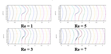
Figure 7. Velocity profiles in different positions along the channel
Figure 7 shows the velocity distribution throughout the channel and across the obstacle, for different Reynolds numbers and nanofluid volume fractions. It is noted that the laminar flow of the nanofluid was almost identical to that of the base fluid (water) as all profile curves coincided, regardless of the Reynolds number. Furthermore, the effect of the volume fraction was noticeable for Re = 7, particularly in the immediate vicinity of the structure.
In addition, the velocity profile showed the same parabolic shape along the channel, where the maximum was registered at the level of the horizontal axis. However, these maxima appeared close to the upper wall of the channel, at the level the obstacle (0.75 < X * <2), as shown by Figure 7.
As Reynolds number increased, Figure 8 showed a widening in the vortex zone downstream of the structure, along an absolute stagnation zone occurring for large inertia forces. This is noticeable at X* = 1.25 position, downstream of the structure, where the velocity in this zone formed a straight line (zero) at Re = 7.
Figure 8. Velocity profile along the axis of the channel
Figure 8 shows the effects of volume fraction and inertia on the axial velocity, along the median longitudinal line of the channel, for Reynolds numbers of 1, 3, 5, and 7. In general, the increase in Reynolds number was associated with an increase in velocity throughout the channel. On the other hand, regardless of Reynolds number, an increase in velocity was observed between the nanofluid entry and the upstream of the structure. A sharp drop was then noticed immediately after the obstacle, interpreted by the existence of recirculation in this zone. The velocity seemed to have then stabilized again at its initial pace beyond the obstacle, but with a sharp increase nearby the end of the channel.
As for the effect of the alumina nanoparticles effect on the axial velocity profile, this was only observed upon the increase in Reynolds number, ergo, upon an increase in the entrance velocity to the pipeline. In particular, a more nanoparticles concentrated fluid was associated with a relative decrease in axial velocity.
4.2 Pressure distribution
In this subsection, the effects of the nanoparticles addition on the hydrodynamic behavior of the nanofluid, as well as on the mechanical behavior of the structure represented by the baffle, were investigated. It is noted that the ultimate goal of this study was to investigate the effect of the concentration of nanoparticles on the deformation of the presented obstacle, which all prior studies hitherto lacks.
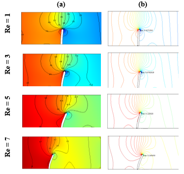
Figure 9 shows the pressure distribution and iso-pressure lines in the structure, for a nanofluid with 4% alumina nanoparticles concentration, and for several Reynolds numbers. A noticeable decrease in pressure was observed upon the increase in Reynolds number. On the other hand, pressure recorded the highest values upstream of the deformed structure, particularly at the bottom of the pipe.
Figure 9. Pressure profiles. (a) Pressure and (b) Iso-pressure lines
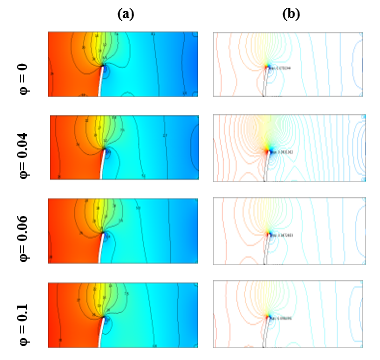
Figure 10. Pressure profiles. (a) Pressure and (b) Iso-pressure lines
Figure 10 shows the pressure distribution and iso-pressure lines in the structure, for different nanoparticles volume fractions, and at Re = 3. Ultimately, an increase in the volume fraction was highly associated with an increase in the nanofluid pressure.
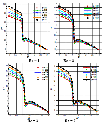
Figure 11 presents the pressure distribution, as a function of the structure entry length, for different volume fractions. In general, the nanofluid laminar flow was characterized by a pressure drop for all Reynolds values. Interestingly, this was a sudden drop after the obstacle. The upstream pressure then exhibited a linear behavior for low Reynolds number.
On the other hand, the increase in the nanofluid alumina concentration was associated with an increase in the fluid pressure, especially at the entrance to the channel.
Figure 11. Nanofluid pressure distribution along the axis of the channel
4.3 Maximum structure displacement
Figure 12 represents the strain of the structure for φ = 4% and for different Reynolds numbers. The maximum displacement has been observed at the free end of the structure. In addition, the increase in Reynolds number, Re, was associated with an increase in strain. This was due to the increase in flow intensity, upstream of the structure, which in turn affected the wall stresses.
On the other hand, Figure 13 represents the strain of the structure for Re = 3 and for different nanoparticles volume fractions (φ). Upon fixing Reynolds number, the maximum recorded displacement was at the free end of the structure. It also increased with increasing the volume fraction, but at a slower pace than that of the Reynolds number case.
The major contribution in this study was to investigate the effects of Reynolds number and nanoparticles volume concentration on the deformation of the structure. As such, for design purposes, it seemed desirable for the authors to add a mathematical relation, based on the current results, allowing to determine the maximum design displacement of the structure as a function of both, Reynolds number and nanoparticles volume fraction represented in Table 4. To obtain this, the least squares and Lagrange interpolation methods were adopted:
In order to give a mathematical character to the present numerical simulations, a correlation between the maximum displacement of the structure, the Reynolds number and the volume fraction of the nanoparticles was made by the use of least squares method.
Figure 12. Deformation of the metallic structure and displacement vectors for different Re
Figure 13. Deformation of the metallic structure and displacement vectors for different φ
Table 4. Maximum displacement of the structure [×10-2]
|
Volume fractions |
Re = 1 |
Re = 3 |
Re = 5 |
Re = 7 |
|
0.00 |
2.58 |
7.55 |
12.06 |
15.97 |
|
0.02 |
2.71 |
7.92 |
12.59 |
16.59 |
|
0.04 |
2.85 |
8.31 |
13.15 |
17.23 |
|
0.06 |
3.01 |
8.72 |
13.73 |
17.90 |
|
0.08 |
3.17 |
9.17 |
14.35 |
18.60 |
|
0.10 |
3.35 |
9.64 |
15.00 |
19.32 |
The maximal displacement is given by:
${{d}_{\max }}\left( \operatorname{Re},\varphi \right)={{f}_{1}}\left( \operatorname{Re} \right)\varphi +{{f}_{2}}\left( \operatorname{Re} \right)$ (15)
With
${{f}_{1}}\left( \operatorname{Re} \right)=\alpha {{\operatorname{Re}}^{^{2}}}+\beta \operatorname{Re}+\gamma $ and ${{f}_{2}}\left( \operatorname{Re} \right)=\xi \operatorname{Re}+\eta $ (16)
Thus, the maximum strain can be expressed as:
$\begin{align} & {{d}_{\max }}\left( \operatorname{Re},\varphi \right)=-0.005{{\operatorname{Re}}^{2}}\varphi +0.088\operatorname{Re}\varphi \\ & +0.022\operatorname{Re}+0.005\varphi +0.006 \\\end{align}$ (17)
This study focused on the effects of fluid flow, particularly suspensions such as nanofluid, on the behavior of a submerged structure. The objective was mainly to study the effects of nanoparticles volume concentration and Reynolds number on the behavior of the structure. The solid and fluid models were treated as two complementary domains, where by their mechanical properties, such as deformation, are governed by the fluid-structure interaction they undergo. Without modifying the intrinsic topology of the mesh of each of these two domains, the nodes can properly displace without going through a systematic remeshing. The solid was modeled via a Lagrangian formulation, whereby the associated mesh was free to displace according to its current position. For a well-defined rigidity (Assigned Young's modulus), the deformation of the structure depended on the nature of the flow, which in turn exerted pressure load son the structure. Results showed that this deformation increased as a result of increasing either of both, Reynolds number and nanoparticles volume fraction.
|
L |
height of the canal |
|
H |
Fin length |
|
W |
displacement vector |
|
E |
dimensional Young’s modulus |
|
Fv |
vector of volume force |
|
P |
pressure filed |
|
Re |
Reynolds number |
|
t |
time in dimensional form |
|
cp |
specific heat, (J kg-1 K-1) |
|
u, v |
Velocity components |
|
U,V |
Dimensionless velocity components |
|
x, y |
Cartesian coordinates |
|
Greek symbols |
|
|
α |
coefficient of the thermal diffusivity (m2.s-1) |
|
β |
coefficient of the volumetric thermal expansion K-1 |
|
σ |
field of the tensor of stress |
|
τ |
dimensionless time |
|
φ |
fraction volumique |
|
μ |
the fluid’s dynamic viscosity |
|
$v$ |
Poisson’s ratio |
|
ρ |
Density (kg m-3) |
|
$\rho_{p}$ |
the ratio of fluid to solid-structure density |
|
Subscripts |
|
|
f |
the fluid property |
|
h |
the hot property |
|
nf |
nanofluid |
[1] Mehryan, S., Chamkha, A., Ismael, M., Ghalambaz, M. (2017). Fluid–structure interaction analysis of free convection in an inclined square cavity partitioned by a flexible impermeable membrane with sinusoidal temperature heating. Meccanica, 52: 2685-2703. https://doi.org/10.1007/s11012-017-0639-8
[2] Ghalambaz, M., Jamesahar, E., Ismael, M.A., Chamkha, A.J. (2017). Fluid-structure interaction study of natural convection heat transfer over a flexible oscillating fin in a square cavity. International Journal of Thermal Sciences, 111: 256-273 https://doi.org/10.1016/j.ijthermalsci.2016.09.001
[3] Shahabadi, M., Mehryan, S.A.M., Ghalambaz, M., Ismael, M. (2020). Controlling the natural convection of a non-Newtonian fluid using a flexible fin. Applied Mathematical Modeling, 92: 669-686. https://doi.org/10.1016/j.apm.2020.11.029
[4] Nithyadevi, N., Kandaswamy, P., Lee, J. (2007). Natural convection in a rectangular cavity with partially active side walls. International Journal of Heat and Mass Transfer, 50: 4688-4697. https://doi.org/10.1016/j.ijheatmasstransfer.2007.03.050
[5] Berry, J.G., Reissner, E. (1958). The effect of an internal compressible fluid column on the breathing vibration of a thin pressurized cylindrical shell. Journal of Aerospace Science, 25: 288-294. https://doi.org/10.2514/8.7643
[6] Coale, C.W., Nagano, M. (2012). Ax symmetric modes of an elastic cylindrical-hemispherical tank partially filled with a liquid. Symposium on structural dynamics and Aero Elasticity. https://doi.org/10.2514/6.1965-1117
[7] Paidoussis, M.P., Grinevich, E., Adamovic, D., Semler, C. (2002). Linear and nonlinear dynamics of cantilever cylinders in axial flow. Part 1: Physical Dynamics. Journal of Fluids and Structure, 16(6): 691-713. https://doi.org/10.1006/jfls.2002.0447
[8] Paıdoussis, M.P., Li, G.X. (1993). Pipes conveying fluid: a model dynamical problem. Journal of Fluids and Structures, 7: 137-204. https://doi.org/10.1006/jfls.1993.1011
[9] Lindholm, U.S., Kana, D.D., Abramson, H.N. (2012). Breathing vibrations of a circular cylindrical shell with an internal liquid. Journal of the Aerospace Sciences, 29(9): 1052-1059. https://doi.org/10.2514/8.9693
[10] Lakis, A.A., Paidoussis, M.P. (1971). Free vibration of cylindrical shells partially filled with liquid. Journal of Sound and Vibration, 19(1): 1-15. https://doi.org/10.1016/0022-60X(71)90417-2
[11] Lindholm, U.S., Kana, D.D., Chu, W.H., Abramson, H.N. (1965). Elastic vibration characteristics of cantilever Plates in water. Journal of Ship Researrch, 9(2): 11-36.
[12] Mittal, S., Tezduyar, T.E. (1995). Parallel fini element simulationof 3D incompressible flow fluid/structure interactions. International Journal for Numerical Methods in Fluids, 21(10): 933-953. https://doi.org/10.1002/fld.1650211011
[13] Messahel, R., Reagan, C., Souli, M., Ruiu, C. (2018). Numerical investigation of homogeneous equilibrium model and fluid-structure interaction for multiphase water flows in pipes. Journal of Multiphase Flow, 98: 56-66. https://doi.org/10.1016/j.ijmultiphaseflow.2017.08.016
[14] Van Loon, R., Anderson, P.D., Baaijens, F.P.T., va de Vosse, F.N. (2005). A three-dimensionna fluid–structure interaction method for heart valve modelling. Comptes Rendus Mécanique, 333(12): 856-866. http://dx.doi.org/10.1016%2Fj.crme.2005.10.008
[15] Goura, G.S.L., Badcock, K.J., Woodgate, M.A., Richards, B.E. (2001). Adata exchange method for fluid-structure interaction problems. The Aeronautical Journal, 105(1046): 215-221. https://doi.org/10.1017/S0001924000025458
[16] Tijsseling, A.S., Lavooij, C.S.W. (1990).Waterhammer with fluid-structure interaction. Appl. Sci. Res., 47: 273-285. https://doi.org/10.1007/BF00418055
[17] Jhung, M.J., Kim, W.T., Ryu, Y.H. (2009). Dynamic characteristics of cylindrical shells considering fluid-structure interaction. Nuclear Engenering and Technology, 41(10): 1333-1346. https://doi.org/10.5516/NET.2009.41.10.1333
[18] Lin, Z.H., Li, X.J., Jin, Z.J., Qian, J.Y. (2020). Fluid-structure interaction analysis on membrane behavior of a microfluidic passive valve. Menbranes, 10(10): 300. https://doi.org/10.3390/membranes10100300
[19] Sigrist, J.F., Lainé, C., Peseux, B. (2005). Modal analysis of an industrial structure with fluid-structure interaction. Mécanique Industries, 6(5): 553-563. https://doi.org/10.1051/meca:2005067
[20] Liu, Z.G., Liu, Y., Lu, J. (2012). Fluid–structure interaction of single flexible cylinder in axial flow. Journal of Computers & Fluids, 56: 143-151. https://doi.org/10.1016/j.compfluid.2011.12.003
[21] Grandmont, C., Maday, Y. (1998). Analysis and numerical method for the simulation of fluid-structure. Interaction Phenomen ESAIM, Procs., 3: 101-117. https://doi.org/10.1051/proc:1998042
[22] De Ridder, J., Degroote, J., Van Tichelen, K., Schuurmans, P., Vierendeels, J. (2013). Modal characteristics of a flexible cylinder in turbulent axial flow from numerical simulations. Journal of Fluids and Structures, 43: 110-123. https://doi.org/10.1016/j.jfluidstructs.2013.09.001
[23] Lin, Y.H., Tsai, Y.K. (1997). Nonlinear vibrations of Timoshenko pipes conveying fluid. International Journal of Solids and Structures, 34(23): 2945-2956. https://doi.org/10.1016/S0020-7683(96)00217-X
[24] Stein, RA., Tobriner, M.W. (1970). Vibration of pipes containing flowing fluids. Journal. Appl. Mechan., 37(4): 906-916. https://doi.org/10.1115/1.3408717
[25] Kohli, A.K., Nakra, B.C. (1984). Vibrations analysis of straight and curved tubes conveying fluid by means of straight beam finite elements. Journal of Sound and Vibration, 93(2): 307-311. https://doi.org/10.1016/0022-460X(84)90314-6
[26] Aldraihem, O.J. (2007). Analysis of the dynamic stability of collar-stiffened pipes conveying fluid. Journal of Sound and Vibration, 300(3-5): 453-465. https://doi.org/10.1016/j.jsv.2006.09.007
[27] Chadi, K., Belghar, N., Guerira, B., Messaoudi, A. (2020). Three-dimensional numerical study of thermal exchanges in different geometry sections of mini-channels using three different nanoparticles. Metallurgical and Materials Engineering, 26(1): 103-119. http://doi.org/10.30544/455
[28] Korib, K., Roudane, M., Khelili, Y. (2020). Numerical study on characteristics of flow and thermal fields around rotating cylinder. Journal of Metallurgical and Materials Engineering, 26(1): 71-86. https://doi.org/10.30544/450
[29] Rao, K.S., Sravani, K.G., Yugandhar, G., Rao, G.V., Mani, V.N. (2015). Design and analysis of fluid structure interaction in a horizontal micro channel. Procedia Materials Science, 10: 768-788. https://doi.org/10.1016/j.mspro.2015.06.022
[30] Sabbar, W.A., Ismael, M.A., Almudhaffar, M. (2018). Fluid-structure interaction of mixed convection in a cavity-channel assembly of flexible wall. International Journal of Mechanical Sciences, 149: 73-83. https://doi.org/10.1016/j.ijmecsci.2018.09.041