Samy M. El-Behery* | Gamal H. Badawy | Fathi M. Mahfouz
© 2022 IIETA. This article is published by IIETA and is licensed under the CC BY 4.0 license (http://creativecommons.org/licenses/by/4.0/).
OPEN ACCESS
This paper presents a numerical study of the turbulent swirling flow in a horizontal tangential inlet tube. The commercial CFD code ANSYS FLUENT 15 was used for solving the set of governing equations using different turbulence models. Eight turbulence models are tested which are, standard k–ε, realizable k–ε, RNG k–ε, SST k–ω, Non-Linear k–ε, v2-f, RSM (Quadratic Pressure-Strain Model), and RSM (Stress-Omega Model). All these turbulence models are available directly in the ANSYS FLUENT except the non-linear k–ε which was implemented in the solver using User Defined Functions (UDF). The numerical predictions are compared with experimental measurements from literature for tangential, axial velocity profiles and Reynolds stresses profiles within the tested tube. The results indicated that the axial velocity is predicted fairly well by the standard k–ε model while the tangential velocity is well predicted by RSM. On the other hand, v2-f model predicts the Reynolds stresses better than the other tested models. The statistical analysis of turbulence model performance showed that, the RSM (Quadratic Pressure-Strain) model gives the best agreement with all data of experiments followed by non-linear k–ε and standard k–ε turbulence models.
turbulence models, swirling flow, CFD, tangential injection
Swirling flows are important class of flows due to their widely used in many engineering applications such as heat exchangers, cyclone separation, mixing, combustion, cooling of gas turbine, etc., and has attracted a widely interest of research due to it’s the strong influence on the flow behavior.
The utilization of swirl imposes rotation imposed on the flow therefore creates a recirculation area, which is essential for some application such as flame stabilization [1-3], reducing the energy losses in a diffuser [4], and heat transfer enhancement [5]. The swirl flow devices can be categorized into two kinds: the continuous swirl flow and decaying swirl flow devices. In the continuous swirl flow devices, the swirling exists over the whole length of the tube such as wire coil and twist tape inserts [5-14], while in the decaying swirl flow devices, the swirl is generated at the entrance of the tube and decays along the flow path such as the tangential flow injection devices, the radial guide vanes and the snail swirl generators [15-24].
In recent years, numerical simulation methods have become essential in many areas of engineering involving internal or external flows. Due to the importance of swirling flows in many engineering applications, it is necessary to identify a particular turbulence model to simulate these flows. Generally, the selection of a turbulence model for particular flow case is governed by the simulation performance and computational time. Despite of the robust performance and the relatively smaller computational effort of the standard k-ε model, it fails to predict the slow decay of eddy viscosity in swirling flows [25]. Kobayashi and Yoda [22] proposed a modified version of the standard k-ε model which considers the eddy viscosity as a tensor instead of scaler quantity. Their results showed that the modified k–ε model successfully predicts the axial and tangential velocity profiles. However, no comparisons were presented for the Reynolds stresses. Gupta and Kumar [23] studied the three-dimensional turbulent swirling flow in a cylinder with tangential inlet and tangential exit using particle tracking velocimetry (PTV) and compared the results with prediction from the standard k-ε and the RNG k-ε turbulence models. Tangential velocity results from the experiments and the RNG k-ε turbulence model were compared and the maximum error is found to be within 20% and these results were considered in reasonably good agreement. In general, the RNG k-ε turbulence model predicted much more accurate results than the standard k-ε model. Saqr et al. [24] used the standard k-ε, the RNG k-ε and a modified version of k-ε model and the results were compared to experimental measurements presented by Gupta and Kumar [23]. The modified k-ε model showed better agreement with the local tangential velocity measurements compared to the standard k-ε and the RNG k-ε turbulence models. Ibrahim et al. [26] compared the performance of standard k–ε model, RNG-based k–ε model, extended k–ε model and low-Reynolds number k–ε model. The results indicated that the RNG-based k–ε model predicted the swirl flow better than other tested models. Ridluan et al. [27] compared the performance of different first order turbulence models (linear eddy viscosity models) in addition to the Reynolds stress model (RSM) in predicting strongly swirling flow. They found that the RSM turbulent model can capture the swirl flow effects better than other models. Norwazan and Jaafar [28] studied high swirling flow using the realizable k–ε model and the results were satisfactory. The performance of the four cubic eddy-viscosity turbulence models for two strongly swirling confined flows were investigated by Yang and Ma [29]. They found that the predicted Reynolds stresses and velocity profiles showed clearly that the superiority of cubic models over the standard k-ε model in the prediction of strongly swirling flows. Shamami and Birouk [30] compared the performance of four two-equation models including standard k–ε, realizable k–ε, RNG k–ε and SST k-ω models along with two Reynolds stress models with linear (RSM) and quadratic (SSG) pressure strain. The comparisons were carried out at two values of swirl number (S=0.4 and S=0.81). They reported that the SSG had the most accurate prediction of mean velocity profiles among the tested models. However, it couldn't predict the magnitude of Reynolds shear stresses. Gorman et al. [31] tested the performance of the standard k–ε, RNG k–ε, standard k-ω and SST k-ω turbulence models in predicting swirling flows. The results were compared to that obtained from LES. They found the SST k-ω turbulence model is the most effective model among the tested two-equation models. The results obtained from LES were closer to the experimental data than any RANS model. On the other hand, the CPU time was 155.3 days for LES and only 14.2 days for SST k-ω. Escue and Cui [32] investigated the swirling flow inside a straight pipe using the commercial CFD code FLUENT. Two-dimensional simulations were performed using the RNG k-ε model and the Reynolds stress model (RSM). The results showed that the RNG k-ε model is in better agreement with experimental velocity profiles for low swirl, while the Reynolds stress model becomes more appropriate as the swirl increases. However, both turbulence models predict an unrealistic decay of the turbulence quantities, indicating the inadequacy of such models in simulating developing pipe flows with swirl. Ćoćić et al. [33] analyzed the efficiency of RNG k-ε, Low-Re k-ε and SST k-ω turbulence models using OpenFOAM CFD software. All the tested eddy viscosity models failed to predict the circumferential velocity. They referred this deficiency to the scaler eddy viscosity of the eddy viscosity model. Therefore, they tested two Reynolds stress models in which the scaler eddy viscosity is not used. They found that the Reynolds stress model with quadratic pressure-strain (SSG model) was more accurate in predicting the main velocity profiles. Unfortunately, no comparisons were made with Reynolds stresses profiles. Liu and Bai [34] investigated the swirl flow generated by short twist tape in a circular pipe using the RNG k-ε and RSM models. They compared the predicted mean flow velocity with measured profiles from literature and they found that the RMS agreed well with the experimental data. On the other hand, Hamdani et al. [35] compared the measured velocity profile with predictions using the RNG k-ε turbulence model and fair agreement was found. Díaz and Hinz [36] investigated the performance of five two-equation turbulence models and they found that the models from k-ε family predicted the swirling flow better than the models from k-ω family. Chin and Philip [37] investigated the three-dimensional swirling flow in a pipe employing direct numerical simulation of the Navier–Stokes and continuity equations. The velocity–vorticity correlations were used that make up the turbulent inertia. Swirling the flow increased the drag and turbulence intensity, and the turbulent inertia decomposition showed that the velocity–vorticity correlations of the axial direction were similar to a 2-D channel flow in the near-wall region. Barakat et al. [38] using Detached Eddy Simulation (DES) calculations and experimental measurements to study the non-reacting swirling behavior through a new double swirl burner. The DES flow fields were compared with high-speed particle image velocimetry (PIV) measurements under different inlet air mass flow rates. It was found that there is a good agreement between the numerical and the experimental results, and the central annular recirculation zone and the corner recirculation zone are well captured. Alahmadi et al. [39] compared the performance of the standard k–ε, RNG k–ε, SST k-ω turbulence models, and the developed shear stress transport model with curvature correction modification (SSTCCM). These models were validated based on experimental data, which represented the flow in a confined cylinder with a rotating lid and the 3D swirling flow through a sudden expansion tube. They found that the SSTCCM model performed well in predicting the axial mean velocity distribution along the longitudinal axis and the axial velocity contours among the tested models. The SSTCCM model was more suitable for capturing the location and extent of the central recirculation zone in the swirling flow immediately after expansion, while other tested models were unable to capture the vortex breakdown phenomenon.
From the previous review it was shown that several two-equation eddy-viscosity models and Reynolds stress models had been evaluated in predicting turbulent swirling flows. Some researchers found the k-ω models especially the SST k-ω turbulence can capture the turbulence swirling flow better than the k-ε models. Whereas, some researchers found the opposite, thus, the RNG k-ε turbulence model was found to perform well by many investigators. On the other hand, many investigators found that the Reynolds stress model can predict the swirling flow better than the eddy-viscosity models. In addition, the four-equation v2-f model was not evaluated in turbulent swirling flow despite of its good performance in flow cases subject to streamline curvature [40, 41]. For the Reynolds stress model, using the specific dissipation rate, ω to determine the length scale instead of the dissipation rate, ε was not evaluated for turbulent swirling flow. Therefore, the aim of present study is to assess the performance of eight turbulence models for turbulent swirling flow including the four-equation v2-f model and the stress-Omega Reynolds stress model. A part of the study is to implement the non-linear k-ε in the FLUENT code and compare its performance with other models.
The commercial computational fluid dynamics (CFD) code ANSYS FLUENT 15 [42] is used for solving the set of governing equations. Different turbulence models were used to predict the turbulent swirling flow in a horizontal tangential inlet tube, which was investigated experimentally by Chang and Dhir [18]. The experiment was conducted by injecting air through four injectors of 15.88 mm inside diameter located on the periphery of an 88.9 mm inside diameter and 1.5 m-long acrylic tube. Eight turbulence models are tested which are, standard k-ε, realizable k-ε, RNG k-ε, SST k-ω, Non-Linear k-ε developed by Ehrhard and Moussiopoulos [43], v2-f, Quadratic pressure-strain Reynolds stress model (SSG), and Stress-Omega Reynolds stress model. All these turbulence models are available directly in the code except the non-linear k-ε model which was implemented in the solver using User Defined Functions (UDF), programmed in C-language. The control volume-based approach is used for discretization the set of governing equations using second order upwind scheme. The SIMPLE algorithm is used for pressure-velocity coupling. The computations are assumed converged when the normalized residual of all governing equations drops below 10-5.
2.1 Governing equations
The steady three-dimensional Reynolds-Average Navier-Stokes (RANS) equations for turbulent incompressible fluid flow with constant properties are used in the present study. The governing equations are the continuity and momentum equations which are given by:
Continuity Equation:
$\frac{\partial u_{i}}{\partial x_{i}}=0$ (1)
Momentum Equation:
$\rho \frac{\partial\left(u_{i} u_{j}\right)}{\partial x_{j}}=-\frac{\partial p}{\partial x_{i}}+\frac{\partial}{\partial x_{j}}\left(\mu \frac{\partial u_{i}}{\partial x_{j}}\right)+\frac{\partial}{\partial x_{j}}\left(-\rho \overline{\acute{u}_{i} \acute{u}_{j}}\right)$ (2)
The term, $\overline{{\acute{u_{i}} \acute{u_{j}}}}$ is called the Reynolds stress tensor and ui and ${\acute{u_{i}}}$ represent the mean and fluctuating velocity component in i-direction, respectively. These equations are not a closed set and turbulence model is required to model the Reynolds stress tensor.
2.2 Turbulence modeling
Some of the used turbulence models are based on the Boussinesq hypothesis which are, standard k-ε, realizable k-ε, RNG k-ε, SST k-ω and v2-f. The Boussinesq hypothesis assumes that the Reynolds stress tensor is proportional linearly to the velocity gradient and it is given by
$\overline{{\acute{u_{i}} \acute{u_{j}}}}=-v_{t}\left(\frac{\partial u_{i}}{\partial x_{j}}+\frac{\partial u_{j}}{\partial x_{i}}\right)+\frac{2}{3} k \delta_{i j}$ (3)
The RSM models solve the Reynolds stresses transport equations individually. The term of the pressure strain in this model can be modelled according to Quadratic Pressure-Strain Model (SSG) or Stress-Omega Model which uses the specific dissipation rate equation for the length scale instead of the dissipation rate equation. To reserve space, one can refer to ANSYS theory guide [42] for detailed description of all above models.
For the non-linear k-ε, the equations of turbulent kinetic energy, k and the dissipation rate, ε are the same as those of the standard k-ε model, while the relationship between the Reynolds stress and velocity gradient (strain rate) is non-linear, this model is based on quadratic stress-strain relationships and can be written as given by Ehrhard and Moussiopoulos [43] as follows:
$\overline{\acute{u}_{i} \acute{u}_{j}}=-2 v_{t} S_{i j}+\frac{2}{3} k \delta_{i j}$
$+C_{1} v_{t} \frac{k}{\varepsilon}\left(S_{i k} S_{k j}-\frac{1}{3} S_{k l} S_{k l} \delta_{i j}\right)$
$+C_{2} v_{t} \frac{k}{\varepsilon}\left(\Omega_{i k} S_{k j}+\Omega_{j k} S_{k i}\right)$
$+C_{3} v_{t} \frac{k}{\varepsilon}\left(\Omega_{i k} \Omega_{j k}-\frac{1}{3} \Omega_{l k} \Omega_{l k} \delta_{i j}\right)$
$+C_{4} v_{t} \frac{k^{2}}{\varepsilon^{2}}\left(S_{k i} \Omega_{l j}+S_{k j} \Omega_{l i}\right) S_{k l}$
$+C_{5} v_{t} \frac{k^{2}}{\varepsilon^{2}}\left(\Omega_{i l} \Omega_{l m} S_{m j}+S_{i l} \Omega_{l m} \Omega_{m j}-\right.$$\left.\frac{2}{3} S_{l m} \Omega_{m n} \Omega_{n l} \delta_{i j}\right)$
$+C_{6} v_{t} \frac{k^{2}}{\varepsilon^{2}} S_{i j} S_{k l} S_{k l}+C_{7} v_{t} \frac{k^{2}}{\varepsilon^{2}} S_{i j} \Omega_{k l} \Omega_{k l}$ (4)
where, Sij and Ωij are the strain and vorticity tensors and defined by:
$S_{i j}=\frac{1}{2}\left(\frac{\partial u_{i}}{\partial x_{j}}+\frac{\partial u_{j}}{\partial x_{i}}\right)$ and $\Omega_{i j}=\frac{1}{2}\left(\frac{\partial u_{i}}{\partial x_{j}}-\frac{\partial u_{j}}{\partial x_{i}}\right)$ (5)
The eddy viscosity νt and the eddy viscosity coefficient Cµ can be written as follows:
$v_{t}=C_{\mu} \frac{k^{2}}{\varepsilon}$
$C_{\mu}=\min \left(\frac{1}{0.9 S^{1.4}+0.4 \Omega^{1.4}+3.5}, 0.15\right)$ (6)
$S=\frac{k}{\varepsilon} \sqrt{2 S_{i j} S_{i j}}, \Omega=\frac{k}{\varepsilon} \sqrt{2 \Omega_{i j} \Omega_{i j}}$ (7)
The constants of the non-linear k-ε model are given in Table 1.
Table 1. Constants of the nonlinear turbulence model
|
C1 |
C2 |
C3 |
−C4 |
C5 |
−C6 |
C7 |
|
-0.2 |
0.4 |
$2 .-e^{-(S-\Omega)^{2}}$ |
$32.0 C_{\mu}^{2}$ |
0.0 |
$16.0 C_{\mu}^{2}$ |
$16.0 C_{\mu}^{2}$ |
2.3 Geometry and computational grids
Figure 1. 3-D geometry and details of injectors from the experiment of Ref. [18]
The test case examined in this study is a 3-D turbulent swirling flow in a horizontal tangential inlet tube, which was investigated experimentally by Chang and Dhir [18]. The experiment was conducted by injecting air through four injectors of 15.88 mm inside diameter placed on the periphery of an 88.9 mm inside diameter and 1.5 m-long tube. The validation results were taken at Reynolds number of 12500 (based on the mean axial velocity and the tube diameter). The details of the geometry of the validation experiments and the mesh are shown in Figures 1 and 2, respectively. The 3-D geometry is modelled by ANSYS design modeller and the structured mesh (quadrilateral cells) is generated using ANSYS meshing. Three different mesh are tested for each turbulence model to ensure grid independent results. These meshes are 400000, 600000 and 900000 cells, respectively. Comparisons between predicted axial velocity profile and experimental results at Z/D=6.06 using the three grids shows that there is no significant difference between 600000 and 900000 cells as shown in Figure 3. Therefore, the results obtained using a computational grid of 600000 cells are presented.
Figure 2. Structured computational grid at mid-length of the tube
Figure 3. Effect of grid resolution on axial velocity profile at Z/D=6.06 for standard k-ε model
2.4 Boundary conditions and wall functions
There are three boundary conditions used in this geometry domain. At the inlet: Velocity inlet boundary condition and is computed from Re=12500. At the outlet: Atmospheric pressure outlet condition is applied. At the wall: The no-slip boundary conditions are specified with wall function approach.
The non-equilibrium wall functions are recommended for use in complex flows involving separation, reattachment, and impingement where the mean flow and turbulence are subjected to pressure gradients and rapid changes [44]. The non-equilibrium wall function is applied to the wall-adjacent cells for the standard k–ε, realizable k-ε, RNG k-ε, non-linear k-ε, RSM (Quadratic Pressure-Strain Model), and RSM (Stress-Omega Model), while the SST k-ω and v2-f models treat the near wall turbulence without the use of wall functions.
The comparisons between present predictions using all the tested turbulence models and the experimental data given by Chang, and Dhir [18] at Re=12500 and Z/D=6.06 for tangential, axial velocities and Reynolds stresses profiles. The radial position is non-dimensionalized by the radius of the pipe, R, while the tangential and axial velocities are normalized by the bulk axial velocity, Uav, and the Reynolds stresses are normalized by $U_{a v}^{2}$.
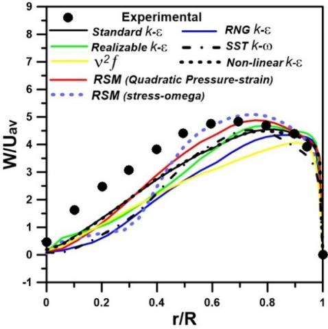
3.1 Tangential velocity
Figure 4 shows a comparison between present predicted and measured radial distribution of tangential velocity profile for all the tested turbulence models. For all turbulence models, the trend of the curve is the same as in the experimental data. That is, the tangential velocity increases with radius in the core region which is characterized by forced vortex and reaches its highest value at about r/R=0.7. The RSM (Quadratic pressure strain) model is the only turbulent model which predicts this high value and its location while the other tested models failed to predict the radial location of the highest tangential velocity. Thereafter, for r/R>0.7, the velocity decreases as the radius increases in the annular region which characterized by free vortex type. Despite the modified dissipation rate equation in the RNG k–ε model and the use of four equations in the v2-f model, they are in a poor agreement with the experimental data. The most accurate model compared with the experimental data is the RSM (Quadratic pressure strain) model followed by standard k–ε and non-linear k–ε. This can be attributed to the anisotropy eddy viscosity in the RSM.
Figure 4. Radial distribution of tangential velocity
3.2 Axial velocity
The radial distribution of axial velocity profiles is presented in Figure 5 for different turbulence models. The figure indicated that the standard k–ε and non-linear k–ε models predict the axial velocity profiles in a good agreement with the experimental data across the entire pipe radius, especially in the region of recirculation (region of negative axial velocity). The rest of the models can be considered acceptable except the v2-f model to predict the profile of axial velocity. This figure indicates that the standard k–ε and non-linear k–ε models capture the characteristics of this profile very adequately.
Figure 5. Radial distribution of axial velocity
Figure 6. Radial distribution of axial Reynolds normal stress
3.3 Turbulence quantities
The development of Reynolds normal and shear stresses profiles are presented in Figures 6-11. In Fluent, the Reynolds stresses are available directly for RSM and the developed UDF for the non-linear k–ε model is used to store the calculated the Reynolds stresses in User Defined Memories (UDM). For the other models, a custom field function is used to calculate and store the Reynolds stresses. It can be seen that the RSM (Quadratic Pressure-Strain) and v2-f models predict the normal Reynolds stresses profiles fairly good, while the other models failed to predict it as a result of the isotropic flow, as shown in Figures 6-8. Figure 9 shows that the non-linear k–ε model predicts the axial-tangential Reynolds shear stress profile very well followed by RSM (Quadratic Pressure-Strain) while the other models are in poor agreement. Figure 10 indicates that the results of radial-tangential Reynolds shear stress for the non-linear k–ε, standard k–ε, RSM (Quadratic Pressure-Strain) and v2-f models better than other models. The standard k–ε and v2-f models predict the axial-radial Reynolds shear stress profiles better than other models as cab be seen in Figure 11.
Figure 7. Radial distribution of tangential Reynolds normal stress
Figure 8. Radial distribution of radial Reynolds normal stress
Figure 9. Radial distribution of axial-tangential Reynolds shear stress
Table 2. The average deviation for all parameters
|
Parameter |
Stand. k-ε |
RNG k-ε |
Realizable k-ε |
Non-linear k-ε |
SST k-ω |
v2-f |
RSM (Quadratic Pressure- Strain) |
RSM (stress-omega) |
|
Axial velocity |
0.2677 |
1.1635 |
1.2448 |
0.3156 |
0.7131 |
1.3263 |
0.4002 |
0.5231 |
|
Tangential velocity |
0.2493 |
0.3866 |
0.3022 |
0.2496 |
0.3470 |
0.3602 |
0.1681 |
0.2978 |
|
Tangential normal stress |
0.6213 |
0.7590 |
0.7193 |
0.4046 |
0.6813 |
0.1263 |
0.1550 |
0.6699 |
|
Radial normal stress |
0.5895 |
0.7278 |
0.6767 |
0.3379 |
0.6306 |
0.1260 |
0.1600 |
0.6313 |
|
Axial normal stress |
0.6218 |
0.7510 |
0.7045 |
0.3616 |
0.6563 |
0.0532 |
0.0574 |
0.6174 |
|
Radial-Tangential stress |
0.7546 |
0.9206 |
0.8081 |
0.7032 |
0.7632 |
1.9538 |
0.7407 |
0.8543 |
|
Axial-Tangential stress |
0.9912 |
1.0179 |
1.0186 |
0.5912 |
0.9260 |
0.7773 |
0.7884 |
0.9363 |
|
Axial-Radial stress |
0.5710 |
0.9747 |
0.8768 |
0.8273 |
0.9739 |
1.2698 |
0.9348 |
1.1432 |
|
overall average deviation |
0.5833 |
0.8376 |
0.7939 |
0.4739 |
0.7114 |
0.7491 |
0.4256* |
0.7092 |
Figure 10. Radial distribution of radial-tangential Reynolds shear stress
Figure 11. Radial distribution of axial--radial Reynolds shear stress
From the previous results, it is clear that the tested turbulence models differ in their prediction. Some models give acceptable results for some parameters and give unacceptable results for other. A statistical analysis is required to determine the most accurate turbulence model which gives the mean predicted results compared to the measured data. The average deviation error (AVDE) between prediction and experimental results for the tested turbulence models is calculated by:
$A V D E=\frac{1}{n} \sum_{i=1}^{i=n} A B S\left(\frac{\Phi_{N u m}-\Phi_{E x p}}{\Phi_{E x p}}\right)$ (8)
where, ϕnum and ϕexp are the numerical and experimental values of parameter, ϕ, respectively. The statistical deviation results of all measured data for each turbulence model are shown in Table 2. The table indicates that the RSM (Quadratic Pressure-Strain) model predict results with the smallest deviation and the largest deviation is given by RNG k–ε model.
The turbulent swirling flow in a horizontal tangential inlet tube was investigated numerically using the commercial CFD code ANSYS FLUENT 15. The performance of eight different turbulence models is compared with published experimental data of Chang and Dhir [18]. The standard k–ε, realizable k–ε, RNG k–ε, SST k–ω, Non-Linear k–ε, v2-f, RSM (Quadratic Pressure-Strain Model), and RSM (Stress-Omega Model) were used. All these turbulence models are available directly in the ANSYS FLUENT code except the non-linear k–ε, this model was implemented in the solver using User Defined Functions (UDF). Statistical analysis of turbulence model performance showed that the RSM (Quadratic Pressure-Strain) model indicates the best agreement with all data of experiments followed by non-linear k–ε and standard k–ε turbulence models.
[1] Gupta, A.K., Lilley, D.G., Syred, N. (1984). Swirl flows. Tunbridge Wells.
[2] Poinsot, T., Veynante, D. (2005). Theoretical and Numerical Combustion. RT Edwards, Inc.
[3] El-Asrag, H., Menon, S. (2007). Large eddy simulation of bluff-body stabilized swirling non-premixed flames. Proceedings of the Combustion Institute, 31(2): 1747-1754. https://doi.org/10.1016/j.proci.2006.07.251
[4] Kochevsky, A.N. (2001). Numerical investigation of swirling flow in annular diffusers with a rotating hub installed at the exit of hydraulic machines. J. Fluids Eng., 123(3): 484-489. https://doi.org/10.1115/1.1385384
[5] Eiamsa-ard, S., Promvonge, P. (2005). Enhancement of heat transfer in a tube with regularly-spaced helical tape swirl generators. Solar Energy, 78(4): 483-494. https://doi.org/10.1016/j.solener.2004.09.021
[6] Chaware, P., Sewatkar, C.M. (2019). Flow transitions for flow through a pipe with a twisted tape insert. Journal of Fluids Engineering, 141(11): 111110. https://doi.org/10.1115/1.4043557
[7] Li, P., Liu, Z., Liu, W., Chen, G. (2015). Numerical study on heat transfer enhancement characteristics of tube inserted with centrally hollow narrow twisted tapes. International Journal of Heat and Mass Transfer, 88: 481-491. https://doi.org/10.1016/j.ijheatmasstransfer.2015.04.103
[8] Nanan, K., Thianpong, C., Promvonge, P., Eiamsa-Ard, S. (2014). Investigation of heat transfer enhancement by perforated helical twisted-tapes. International Communications in Heat and Mass Transfer, 52: 106-112. https://doi.org/10.1016/j.icheatmasstransfer.2014.01.018
[9] Farnam, M., Khoshvaght-Aliabadi, M., Asadollahzadeh, M. J. (2018). Heat transfer intensification of agitated U-tube heat exchanger using twisted-tube and twisted-tape as passive techniques. Chemical Engineering and Processing-Process Intensification, 133: 137-147. https://doi.org/10.1016/j.cep.2018.10.002
[10] Khoshvaght-Aliabadi, M., Feizabadi, A., Khaligh, S.F. (2019). Empirical and numerical assessments on corrugated and twisted channels as two enhanced geometries. International Journal of Mechanical Sciences, 157: 25-44. https://doi.org/10.1016/j.ijmecsci.2019.04.026
[11] Li, X., Zhu, D., Yin, Y., Tu, A., Liu, S. (2019). Parametric study on heat transfer and pressure drop of twisted oval tube bundle with in line layout. International Journal of Heat and Mass Transfer, 135: 860-872. https://doi.org/10.1016/j.ijheatmasstransfer.2019.02.031
[12] Khanmohammadi, S., Mazaheri, N. (2019). Second law analysis and multi-criteria optimization of turbulent heat transfer in a tube with inserted single and double twisted tape. International Journal of Thermal Sciences, 145: 105998. https://doi.org/10.1016/j.ijthermalsci.2019.105998
[13] Samruaisin, P., Kunlabud, S., Kunnarak, K., Chuwattanakul, V., Eiamsa-Ard, S. (2019). Intensification of convective heat transfer and heat exchanger performance by the combined influence of a twisted tube and twisted tape. Case Studies in Thermal Engineering, 14: 100489. https://doi.org/10.1016/j.csite.2019.100489
[14] Kumar, B., Kumar, M., Patil, A.K., Jain, S. (2019). Effect of V cut in perforated twisted tape insert on heat transfer and fluid flow behavior of tube flow: An experimental study. Experimental Heat Transfer, 32(6): 524-544. https://doi.org/10.1080/08916152.2018.1545808
[15] Blum, H.A., Oliver, L.R. (1967). Heat transfer in a decaying vortex system. ASME Paper No. 66-WA/HT-62.
[16] Hay, N., West, P.D. (1975). Heat transfer in free swirling flow in a pipe. Journal of Heat Transfer, 97: 411-416. https://doi.org/10.1115/1.3450390
[17] Kitoh, O. (1991). Experimental study of turbulent swirling flow in a straight pipe. Journal of Fluid Mechanics, 225: 445-479. https://doi.org/10.1017/S0022112091002124
[18] Chang, F., Dhir, V.K. (1994). Turbulent flow field in tangentially injected swirl flows in tubes. International Journal of Heat and Fluid Flow, 15(5): 346-356. https://doi.org/10.1016/0142-727X(94)90048-5
[19] Chang, F., Dhir, V.K. (1995). Mechanisms of heat transfer enhancement and slow decay of swirl in tubes using tangential injection. International Journal of Heat and Fluid Flow, 16(2): 78-87. https://doi.org/10.1016/0142-727X(94)00016-6
[20] Yilmaz, M., Çomakli, Ö., Yapici, S. (1999). Enhancement of heat transfer by turbulent decaying swirl flow. Energy Conversion and Management, 40(13): 1365-1376. https://doi.org/10.1016/S0196-8904(99)00030-8
[21] Durmuş, A., Durmuş, A., Esen, M. (2002). Investigation of heat transfer and pressure drop in a concentric heat exchanger with snail entrance. Applied Thermal Engineering, 22(3): 321-332. https://doi.org/10.1016/S1359-4311(01)00078-3
[22] Kobayashi, T., Yoda, M. (1987). Modified k-ε model for turbulent swirling flow in a straight pipe: Fluids engineering. JSME International Journal, 30(259): 66-71. https://doi.org/10.1299/jsme1987.30.66
[23] Gupta, A., Kumar, R. (2007). Three-dimensional turbulent swirling flow in a cylinder: Experiments and computations. International Journal of Heat and Fluid Flow, 28(2): 249-261. https://doi.org/10.1016/j.ijheatfluidflow.2006.04.005
[24] Saqr, K.M., Aly, H.S., Wahid, M.A., Sies, M.M. (2009). Numerical simulation of confined vortex flow using a modified k-ϵ turbulence model. CFD Letters, 1(2): 87-94.
[25] Hamba, F. (2017). History effect on the Reynolds stress in turbulent swirling flow. Physics of Fluids, 29(2): 025103. https://doi.org/10.1063/1.4976718
[26] Ibrahim, K.A., Hamed, M.H., El-Askary, W.A., El-Behery, S.M. (2013). Swirling gas–solid flow through pneumatic conveying dryer. Powder Technology, 235: 500-515. https://doi.org/10.1016/j.powtec.2012.10.032
[27] Ridluan, A., Eiamsa-ard, S., Promvonge, P. (2007). Numerical simulation of 3D turbulent isothermal flow in a vortex combustor. International Communications in Heat and Mass Transfer, 34(7): 860-869. https://doi.org/10.1016/j.icheatmasstransfer.2007.03.021
[28] Norwazan, A.R., Jaafar, M. (2015). Significant of isothermal flow studies for high swirling flow in unconfined burner. Applied Mechanics and Materials, 789: 477-483. https://doi.org/10.4028/www.scientific.net/AMM.789-790.477
[29] Yang, X., Ma, H. (2003). Computation of strongly swirling confined flows with cubic eddy-viscosity turbulence models. International Journal for Numerical Methods in Fluids, 43(12): 1355-1370. https://doi.org/10.1002/fld.565
[30] Shamami, K.K., Birouk, M. (2008). Assessment of the performances of RANS models for simulating swirling flows in a can-combustor. The Open Aerospace Engineering Journal, 1(1): 8-27. http://dx.doi.org/10.2174/1874146000801010008
[31] Gorman, J.M., Sparrow, E.M., Abraham, J.P., Minkowycz, W.J. (2016). Evaluation of the efficacy of turbulence models for swirling flows and the effect of turbulence intensity on heat transfer. Numerical Heat Transfer, Part B: Fundamentals, 70(6): 485-502. https://doi.org/10.1080/10407790.2016.1244390
[32] Escue, A., Cui, J. (2010). Comparison of turbulence models in simulating swirling pipe flows. Applied Mathematical Modelling, 34(10): 2840-2849. https://doi.org/10.1016/j.apm.2009.12.018
[33] Ćoćić, A.S., Lečić, M.R., Čantrak, S.M. (2014). Numerical analysis of axisymmetric turbulent swirling flow in circular pipe. Thermal Science, 18(2): 493-505. https://doi.org/10.2298/TSCI130315064C
[34] Liu, W., Bai, B. (2015). A numerical study on helical vortices induced by a short twisted tape in a circular pipe. Case Studies in Thermal Engineering, 5: 134-142. https://doi.org/10.1016/j.csite.2015.03.003
[35] Hamdani, A., Ihara, T., Kikura, H. (2016). Experimental and numerical visualizations of swirling flow in a vertical pipe. Journal of Visualization, 19(3): 369-382. https://doi.org/10.1007/s12650-015-0340-8
[36] Díaz, D.D.O., Hinz, D.F. (2015). Performance of eddy-viscosity turbulence models for predicting swirling pipe-flow: Simulations and laser-doppler velocimetry. arXiv preprint arXiv:1507.04648.
[37] Chin, R.C., Philip, J. (2021). Swirling turbulent pipe flows: Inertial region and velocity–vorticity correlations. International Journal of Heat and Fluid Flow, 87: 108767. https://doi.org/10.1016/j.ijheatfluidflow.2020.108767
[38] Barakat, S., Wang, H., Jin, T., Tao, W., Wang, G. (2021). Isothermal swirling flow characteristics and pressure drop analysis of a novel double swirl burner. AIP Advances, 11(3): 035240. https://doi.org/10.1063/5.0041361
[39] Alahmadi, Y.H., Awadh, S.A., Nowakowski, A.F. (2021). Simulation of swirling flow with a vortex breakdown using modified shear stress transport model. Industrial & Engineering Chemistry Research, 60(16): 6016-6026. https://doi.org/10.1021/acs.iecr.1c00158
[40] El-Behery, S.M., Hamed, M.H. (2011). A comparative study of turbulence models performance for separating flow in a planar asymmetric diffuser. Computers & Fluids, 44(1): 248-257. https://doi.org/10.1016/j.compfluid.2011.01.009
[41] Balabel, A., Hegab, A.M., Nasr, M., El-Behery, S.M. (2011). Assessment of turbulence modeling for gas flow in two-dimensional convergent–divergent rocket nozzle. Applied Mathematical Modelling, 35(7): 3408-3422. https://doi.org/10.1016/j.apm.2011.01.013
[42] FLUENT 15 Theory Guide, ANSYS Inc. (2013).
[43] Ehrhard, J., Moussiopoulos, N. (2000). On a new nonlinear turbulence model for simulating flows around building-shaped structures. Journal of Wind Engineering and Industrial Aerodynamics, 88(1): 91-99. https://doi.org/10.1016/S0167-6105(00)00026-X
[44] Kim, S., oudhury, D. (1995). A near-wall treatment using wall functions sensitized to pressure gradient. American Society of Mechanical Engineers, Fluids Engineering Division (Publication) FED, 217: 273-280.