Yong Dong | Ruiquan Liao | Wei Luo | Mengxia Li*
© 2022 IIETA. This article is published by IIETA and is licensed under the CC BY 4.0 license (http://creativecommons.org/licenses/by/4.0/).
OPEN ACCESS
Compared with experimental data of pressure drop of gas-liquid two-phase upward flow with low gas-liquid ratio in vertical pipe, the mean relative error of pressure drop predicted by Orkiszewski’s model is 63.62%, the maximum relative error of the model is 98.07%. This paper first introduces the process of acquiring experimental data, then, combined with the experimental data, it is pointed out that the Orkiszewski’s model has a small error in predicting the annular-mist flow pattern, but a large error in predicting the slug flow pattern and annular-slug transition flow pattern. The author analyzes the structure of Orkiszewski’s model and points out that the formula of liquid distribution coefficient in slug flow pattern is complex and very important. In this paper, a new threshold value of liquid distribution coefficient is proposed and an improved Orkiszewski’s model is obtained by particle swarm optimization. The calculated results of experimental data show that the average relative error of the new model is reduced to 25.28%, and the average relative error of the new model can be reduced from 76.17% to 17.21% for the slug flow pattern with continuous oil phase and total flow velocity greater than or equal to 3.048m/s.
gas-liquid two-phase upward flow, vertical pipe, low gas-liquid ratio, pressure drop prediction, Orkiszewski’s model, liquid distribution coefficient
Effective prediction of pressure drop of multiphase pipe flow is an important theoretical basis for design and analysis of oil and gas wells. Much research has been carried out [1-4] in the field. As we all know, Orkiszewski's model is a representative prediction model for pressure drop of multiphase flow in vertical pipe based on flow regime division. The model is obtained by optimizing and combining multiple models. such as Grifitth [5] and Duns [6]. Orkiszewski's calculation of data from 148 actual wells showed an average error of -0.8% [7]. The model is widely accepted [8-19]. Pourafshary et al. [8] obtained the multiphase flow simulator of composite wellbore/reservoir by combining reservoir simulator and wellbore simulator, The Orkiszewski’s model is a branch algorithm of the simulator. Li et al. [9] combined the traditional multiphase flow correlation with artificial neural network to obtain a prediction model with a new structure. Orkiszewski’s model is also a branch algorithm of the simulator. Abd El et al. [10] analyzed the prediction accuracy of the correlation relation in different well conditions and pointed out that in some well conditions, the predicton error of Orkiszewski’s model was the least. Al-Ruhaimani et al. [11] analyzed the influence of high liquid viscosity on flow pattern, pressure gradient and liquid holdup of Orkiszewski’s model. Akinsete and Adesiji [12] pointed out that Orkiszewski’s model is very popular and widely used. Waltrich et al. [13] compared the prediction errors of a variety of prediction models based on experimental data, indicating that the average relative error of Orkiszewski’s model on some data exceeded 50%. Opoku et al. [14] pointed out that Orkiszewski’s model is especially suitable for situations with large fluctuation range of gas-liquid ratio, such as gas-lift process. Luo et al. [15], Chaari et al. [16] pointed out that Orkiszewski’s model contains a large number of parameters, and it is recommended not to exceed the application range. Al Shehri et al. [17] pointed out in 2020 that the Orkiszewski’s model is still an important and widely accepted pressure drop prediction formula. Bogachev et al. [18, 19] regard Orkiszewski’s model as an optional algorithm of solver.
The calculation results based on experimental test data show that the average relative error between the pressure drop predicted by Orkiszewski’s model and the measured pressure drop is 63.62%, and the average relative error reaches 76.17% for the continuous oil phase slug flow pattern. Therefore, it is necessary to further study Orkiszewski's model to improve the prediction accuracy of pressure drop.
This paper first introduces the process of acquiring experimental data, analyzes the structure of Orkiszewski’s model, and points out that the calculation process of liquid distribution coefficient is very complicated and very important. Then a new calculation method of liquid distribution coefficient is proposed and a new model is obtained. The experimental results show that the new model reduces the average relative error to 25.99%.
Experimental data are from the multiphase flow experimental platform, and the components of the platform equipment are shown in the Figure 1.
Figure 1. System construction drawing (Meaning of codes, 1. oil inlet; 2. water inlet; 3. oil-water mixing tank; 4. liquid pump; 5. pressure gage; 6. regulating valve; 7. moisture content meter; 8. fluid flowmeter; 9. regulating pressure valve; 10. gas and liquid mixer; 11. drain pipe; 12. quick shut-off valve; 13. differential pressure pickup; 14. stainless steel barrel part; 15. glass steel tube observation section; 16. Valve; 17. gas-liquid separator)
The experimental scheme is described below. The inside diameter of vertical pipe is 75 mm. The liquid volume flow consists of 10, 15,20,30,40,50 m3/d (Water cut is 0%). Gas liquid ratio consists of 50,100,150,200,300m3/m3. The temperature range during the experiment is between 27 degrees Celsius and 29 degrees Celsius. The fluid medium is air and 5# white oil. There are 30 groups of experimental data.
During the experiment, first control the gas flow and liquid flow as close as possible to the design value according to the experimental design scheme. When the system runs smoothly enough, record the flow pattern (naked eye recognition), close the quick shut-off valves, and place the pipe in a horizontal position. When the oil/gas interface is stable, record the liquid height from the observation part of the glass steel cylinder, and convert the height to the liquid holdup.
Then, the recorded data include: liquid flow, liquid holdup, gas flow, temperature, pressure drop, flow regime.
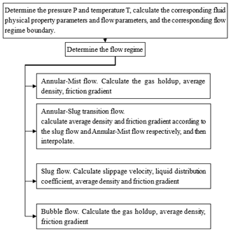
The prediction process of Orkiszewski’s model [5, 20, 21] is shown in the Figure 2.
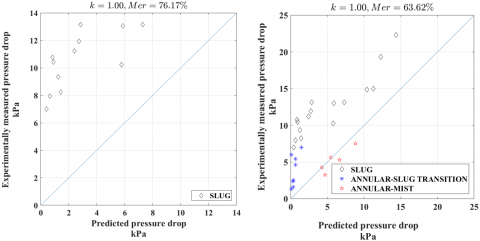
Classify data by flow regime according to flow regime rules. The measured data is taken as the ordinate and the predicted value as the abscissa to make a comparison, as shown in Figure 3.
Figure 2. Simple prediction scheme Orkiszewski's model
Figure 3. Comparison between measured pressure drop and predicted pressure drop
In Figure 3, black diamond corresponds to slug flow regime, blue star corresponds to annular-slug transition flow regime, red pentagram corresponds to annular-mist flow regime, and the line segment from bottom left to top right corresponds to the locus of points where the predicted pressure drop is equal to the test pressure drop. it should be noted that no point corresponds to bubble flow regime. Obviously, red pentagram has small error, but black diamond and blue star has fairly big error. It is noted that the pressure drop prediction model of annular-slug transition flow regime is weighted average by the prediction model of slug flow regime and the prediction model of annular-mist flow regime, therefore, it is very important to improve the prediction accuracy of pressure drop of slug flow regime.
Perform quantitative analysis on the data in Figure 3. Firstly, define relative error as Eq (1):
$e v=\left|\frac{m v-p v}{m v}\right| \times 100 \%$ (1)
where, mv represents the measured value, MPa; pv represents the predicted value, MPa; $|\cdot|$ means take the absolute value operation.
The mean of the relative error of the experimental data points is called the mean relative error, denoted as Mer. For Figure 3, Mer is 63.26%, it indicates that the prediction error of pressure drop is fairly big.
In the slug flow pressure drop prediction model, the calculation process of liquid distribution coefficient is the most complex, as shown in Figure 4.
The complexity of calculation process shows the importance of liquid distribution coefficient, so we can try to improve the prediction model from the perspective of liquid distribution coefficient.
Figure 4. Calculation process of liquid distribution coefficient C0
In the experimental data, the water cut is 0%, which belongs to the continuous oil phase. Sixteen data points are identified as slug flows by the Orkiszewski's model, among which 12 data points have a total velocity greater than the threshold of 3.048m/s. Therefore, in this paper, the improvement of the prediction model of pressure drop of slug flow pattern in Orkiszewski's model mainly focuses on Formula 2 and threshold 2 in Figure 4.
For slug flow in Orkiszewski’s model, when the oil phase is continuous and the total flow rate is greater than or equal to 3.048m/s, the calculation formula of the liquid distribution coefficient is as follows Eq (2) [6, 7]:
$C_{0}=\left[0.00537 \times \log _{10}\left(1000 \mu_{l}+1\right)\right] / D^{1.371}$$+0.455+0.569 \times \log _{10} D-\left(\log _{10} v_{t}+0.516\right)\left\{\left[0.0016 \times \log _{10}\left(1000 \mu_{l}+1\right)\right] / D^{1.571}\right.$$\left.+0.722+0.63 \log _{10} D\right\}$ (2)
where, $\mu_1$ represents liquid viscosity, $P a \bullet S$; D represents pipe Inner Diameter, m; vt represents total velocity of gas-liquid mixture, m/s.
The 2_th threshold value $t v_{2}$ is as follows Eq (3):
$t v_{2}=-\frac{v_{s} A}{Q+v_{s} A}\left(1-\frac{\rho_{m}}{\rho_{l}}\right)$ (3)
if C0<tv2
then set C0=tv2
where, tv2 represents the 2_th threshold value; vs represents slippage velocity, m/s; A represents pipeline sectional area, m2; Q represents total volume flow, m3/s; rm represents average density of gas-liquid mixture, kg/m3; rl represents density of liquid, kg/m3.
Make the following changes:
$t v_{2}^{\prime}=k \cdot t v_{2}$ (4)
if $C_{0}<t v_{2}^{\prime}$
then set $C_{0}=t v_{2}^{\prime}$
where, k is scale factor.
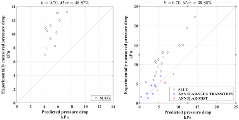
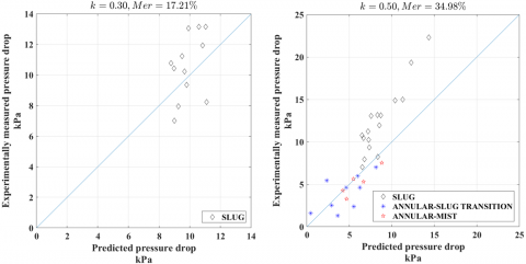
The following figure shows the influence of different values of k on the predicted pressure drop under the slug flow pattern and on the overall experimental data.
Figure 5. Comparison diagram of prediction effect corresponding to different k values (The title of the figure is k value and corresponding mean relative error)
In Figure 5, the total flow velocity corresponding to the data points in the left figure is greater than or equal to 3.048m/s, and both are slug flow patterns. It is easy to see that when k=0.3, the new model improves the predicted pressure drop the most, and the average relative error decreases to 17.21%, and the average relative error decreases by about 59%. The figure on the right shows the comparison of the prediction effect of the new model when k is taken with different values. It is easy to see that when k=0.5, the average relative prediction error is the smallest, which is 34.98%, decreasing by 29%.
In Figure 5, the optimal value k=0.3 corresponding to the left figures is inconsistent with the optimal value k=0.5 corresponding to the right figures, because as shown in Fig. 4, The Orkiszewski’s model under the annular-slug transition flow regime uses the prediction formula of slug flow regime, and the improved fluid distribution coefficient for the slug flow regime will affect the pressure drop prediction effect of annular-slug transition flow regime.
It is similar to the improvement method made in formula (4), for slug flow with continuous oil phase and total flow velocity greater than or equal to 3.048m/s. For continuous oil phase with total flow velocity less than 3.048m/s, introducing scale factor k0=0.1 for threshold value. For annular-slug transition flow regime, continuous oil phase, the total flow rate is less than 3.048m/s, introducing scale factor k0’=1 for threshold value. For annular-slug transition flow regime, continuous oil phase, the total flow rate is greater than or equal to 3.048m/s, introducing scale factor k’=0.55 for threshold value.
Figure 6. Multi-scale factors improved model prediction effect drawing
When k0=0.1, k0’=1, k=0.2 and k’=0.55, the prediction effect of the improved Orkiszewski’s model is shown in the Figure 6.
The average relative error of the new model is 25.99%. Compared with the original model, the average relative error decreased by 50.18%.
The objective function to be optimized is:
$\min \operatorname{Mer}\left(k, k^{\prime}, k 0, k 0^{\prime}\right)$ s.t. $\left\{\begin{array}{l}0.05 \leq k \leq 1.3 \\ 0.05 \leq k^{\prime} \leq 1.3 \\ 0.05 \leq k 0 \leq 1.3 \\ 0.05 \leq k 0^{\prime} \leq 1.3\end{array}\right.$
Standard particle swarm optimization (PSO) algorithm is adopted, and its pseudo-code is shown in Figure 7.
Figure 7. Pseudo-code of standard particle swarm optimization
where,
N: population size
max_gen: maximum generations
k: generation counter from 1 to max_gen
i: particle’s id counter from 1 to N
pBesti: the best previous position of the ith particle
gBest: the best position discovered by the whole population
d: dimension
$X_{i}^{d}: i^{t h}$ particle’s dth dimension’s value of position
$V_{i}^{d}: i^{t h}$ particle’s dth dimension’s value of velocity
$\omega$: inertia weight $\left(\omega_{0}=0.9, \omega_{1}=0.2\right)$
c1=c2=2: learning factor
$\operatorname{rand} 1_{i}^{d}, \operatorname{rand} 2_{i}^{d}$: random numbers in the range [0, 1]
The optimized parameters are: k=0.05, k0=0.25, k’=0.678, k0’=0.845, The average relative error of the new model is 25.28%. The prediction effect is similar to that of the model in section 5.
(1) Based on the experimental data of vertical pipe upward multiphase flow, the prediction error of the improved Orkiszewski’s model decreases to 25.28%, while the original form is 63.26%.
(2) In this paper, the threshold value in Orkiszewski’s model is improved by introducing the scale factor, However, the author did not analyze the reasons behind the phenomenon. The next step is to study the mechanism behind the phenomenon.
The authors will thank people in the Branch of Key Laboratory of CNPC for Oil and Gas Production and Laboratory of Multiphase Pipe Flow, Gas Lift Innovation Center, CNPC for their great help. This paper is supported by National Natural Science Foundation of China (Grant No.: 62173049) and Scientific Research Project of Education Department of Hubei Province (Grant No.: D20211302).
[1] Ali, Z., Anuar, A., Grippo, N., Ramli, N.E., Rahim, N. (2021). Unifying of steady state and transient simulations methodologies for increasing oil production of integrated network of wells, pipeline and topside processing equipment. In Abu Dhabi International Petroleum Exhibition & Conference, OnePetro, SPE-207470-MS. https://doi.org/10.2118/207470-MS
[2] Lawrence, E., Loevereide, M.B., Kalidas, S., Le, N.L., Antoneus, S.T., Khanh, T.L.M. (2021). Production optimization in mature field through scenario prediction using a representative network model: A rapid solution without well intervention. In SPE/IATMI Asia Pacific Oil & Gas Conference and Exhibition, OnePetro, SPE-205662-MS. https://doi.org/10.2118/205662-MS
[3] Chaves, G., Monteiro, D., Duque, M.C., Baioco, J., Vieira, B.F. (2021). Short-term production optimization under water-cut uncertainty. SPE Journal, 26(5): 3054-3074. https://doi.org/10.2118/204223-PA
[4] Grifantini, S., Saqib, T., Sabri, A.M., Keshtta, O.M., Albadi, B.S., Beaman, D.J., Bansal, B.D. (2020). Maximizing mature offshore field value by using auto gas lift technique. In Abu Dhabi International Petroleum Exhibition & Conference, OnePetro, SPE-202793-MS. https://doi.org/10.2118/202793-MS
[5] Grifitth, P., Wallis, G.B. (1961). Two-phase slug flow. Transaction of Asme, 83: 307-320.
[6] Duns, H., Ros, N.C.J. (1963). Vertical flow of gas and liquid mixtures in wells. In 6th world petroleum congress. OnePetro, WPC-10132.
[7] Orkiszewski, J. (1967). Predicting two-phase pressure drops in vertical pipe. Journal of Petroleum Technology, 19(6): 829-838. https://doi.org/10.2118/1546-PA
[8] Pourafshary, P., Varavei, A., Sepehrnoori, K., Podio, A. (2008). A compositional wellbore/reservoir simulator to model multiphase flow and temperature distribution. In International Petroleum Technology Conference. OnePetro, IPTC-12115-MS. https://doi.org/10.2523/IPTC-12115-MS
[9] Li, X., Miskimins, J.L., Hoffman, B.T. (2014). A combined bottom-hole pressure calculation procedure using multiphase correlations and artificial neural network models. In SPE Annual Technical Conference and Exhibition. OnePetro, SPE-170683-MS. https://doi.org/10.2118/170683-MS
[10] Abd El Moniem, M., El-Banbi, A.H. (2015). Proper selection of multiphase flow correlations. In SPE North Africa Technical Conference and Exhibition. OnePetro, SPE-175805-MS. https://doi.org/10.2118/175805-MS
[11] Al-Ruhaimani, F., Pereyra, E., Sarica, C., Al-Safran, E.M., Torres, C.F. (2017). Experimental analysis and model evaluation of high-liquid-viscosity two-phase upward vertical pipe flow. SPE Journal, 22(3): 712-735. https://doi.org/10.2118/184401-PA
[12] Akinsete, O., Adesiji, B.A. (2019). Bottom-hole pressure estimation from wellhead data using artificial neural network. In SPE Nigeria Annual International Conference and Exhibition. OnePetro, SPE-19762-MS. https://doi.org/10.2118/198762-MS
[13] Waltrich, P.J., Capovilla, M.S., Lee, W., de Sousa, P.C., Zulqarnain, M., Hughes, R., Griffith, C. (2019). Experimental evaluation of wellbore flow models applied to worst-case-discharge calculations for oil wells. SPE Drilling & Completion, 34(3): 315-333. https://doi.org/10.2118/184444-PA
[14] Opoku, D., Al-Ghamdi, A., Osei, A. (2020). Novel method to estimate bottom hole pressure in multiphase flow using quasi-monte Carlo method. In International Petroleum Technology Conference. OnePetro, IPTC-20080-MS. https://doi.org/10.2523/IPTC-20080-MS
[15] Luo, C., Wu, N., Dong, S., Liu, Y., Ye, C., Yang, J. (2021). Experimental and modeling studies on pressure gradient prediction for horizontal gas wells based on dimensionless number analysis. In SPE Annual Technical Conference and Exhibition. OnePetro., SPE-206047-MS. https://doi.org/10.2118/206047-MS
[16] Chaari, M., Ben Hmida, J., Seibi, A.C., Fekih, A. (2020). An integrated genetic-algorithm/artificial-neural-network approach for steady-state modeling of two-phase pressure drop in pipes. SPE Production & Operations, 35(3): 628-640. https://doi.org/10.2118/201191-PA
[17] Al Shehri, F.H., Gryzlov, A., Al Tayyar, T., Arsalan, M. (2020). Utilizing machine learning methods to estimate flowing bottom-hole pressure in unconventional gas condensate tight sand fractured wells in Saudi Arabia. In SPE Russian Petroleum Technology Conference. OnePetro, SPE-201939-MS. https://doi.org/10.2118/201939-MS
[18] Bogachev, K., Zagainov, A., Piskovskiy, E., Moshina, I., Grishin, A., Muryzhnikov, A., Korostelev, N. (2021). Integrated field development modeling of block in giant oil reservoir. In SPE Russian Petroleum Technology Conference. OnePetro, SPE-206539-MS. https://doi.org/10.2118/206539-MS
[19] Bogachev, K., Grishin, A., Piskovskiy, E., Erofeev, V. (2020). New solution in integrated asset modeling for multi reservoirs coupling. In SPE Russian Petroleum Technology Conference. OnePetro, SPE-201946-MS. https://doi.org/10.2118/201946-MS
[20] Li, Y.C. (2009). Oil Recovery Engineering. Petroleum Industry Press, 44-48.
[21] Wan, R.P. (2000). Oil Recovery Engineering Manual. Petroleum Industry Press, 1: 194-201.