Mohammed Salah Belalem* | Mohammed Elmir | Mohammed Tamali | Razli Mehdaoui | Abdelkrim Missoum | Toufik Chergui | Salah Bezari
© 2021 IIETA. This article is published by IIETA and is licensed under the CC BY 4.0 license (http://creativecommons.org/licenses/by/4.0/).
OPEN ACCESS
In this work, we propose to experimentally and numerically study the natural convection in laminar regime in an agricultural greenhouse located in South West of Algeria and more precisely in the Adrar area. The numerical study is two-dimensional and was carried out on a tunnel greenhouse with an area of 180m2 located in Adrar in the southwest of Algeria (Latitude: 27°52′27″N, longitude: 0°17′37″W, the laltitude above sea level is 257 m), with polyethylene cover and houses two rows of tomato plants. The experimental study was made during the winter or flowering period of tomato plants (February) when the temperature difference outside the greenhouse is maximum: T min = 3℃ at night and T max = 20℃ the day. We used a calculate code based on the finite element method to numerically simulate the phenomenon of heat transfer inside the greenhouse. The results of the numerical simulation are in the form of isotherms, streamlines and variations in temperature and speed in the greenhouse. The value of the temperature calculated by numerical simulation at the position where the sensor has been placed will be compared with that measured by the sensor. It was concluded that to have a favorable environment for the growth of tomatoes, we must keep the openings closed especially during the night without needing a heating system, especially in this region characterized by a hyper arid climate.
greenhouse, plant, tomato, sensor, porous medium, natural convection, numerical simulation, finite elements method
Greenhouse cultivation has undergone quite remarkable development in Algeria, both spatially and technologically, which requires technical and scientific managers to make this essential model a powerful vector for the country's vegetable production. The reason for using the greenhouse is therefore to create climatic conditions that are more favorable than the local climate, in order to allow continuous production of so-called “off-season” crops thanks to a temperature gain by the greenhouse effect under the structure. However, the climate inside greenhouses depends mainly on its ventilation. Its control makes it possible to control the parameters essential to the proper functioning of the greenhouse (temperature, humidity, etc.). In recent years several researchers have conducted numerical modelling studies of greenhouse microclimates using CFD in order to describe the climate and air flow in greenhouses, significant results have been obtained. Among these works we can cite the work of Haxaire et al. [1] who characterized and modelled the air flows induced by natural ventilation in a greenhouse. Their results show that the climate is an essential factor in the physiological activity of plants. Radiation playing a major role in photosynthesis and temperature largely determining their growth and development. Transpiration plays a fundamental role in the movement of water and minerals in plants and it is also highly dependent on the temperature and humidity of the air. Boulard et al. [2] Characterized and modelled the air flows induced by natural ventilation in a greenhouse. The results show that in the absence of sporulation in the greenhouse, the aerial exchange mechanisms between the interior and exterior of the greenhouse are crucial in determining the interior transport and distribution of Botrytis inoculum and the distribution of the interior climate. Draoui et al. [3] studied the natural convection in laminar and transient regime inside a tunnel greenhouse heated from below (flow) not cultivated. They found that, for small temperature differences maintained between the ground and the roof, the air circulation is characterized by two recirculation cells rotating in opposite directions and that the air pressure inside the greenhouse is important near the ground, this allows good air circulation in the greenhouse and supports the idea of placing the openings at the top (at roof level), which has the effect of evacuating or renewing the greenhouse air. Wang et al. [4] investigated air velocity profiles at the center of a naturally ventilated greenhouse with a tomato crop were investigated using a custom multipoint two-dimensional sonic anemometer system. Experimental results showed that the air speed linearly depended on both the external wind speed and the greenhouse ventilation flow. Ould Khaoua et al. [5] analyzed the efficiency of ventilation of greenhouses with CFD the results showed that aeration directly influences the heat and mass transport between the external environment and the interior, thus strongly affecting the prevailing climate in the greenhouse. Bougoul et al. [6] studied the numerical simulation of air movement and temperature variation in heated greenhouses using fluid dynamics software (CFD) to see the influence of heating tubes on air circulation as well as the temperature variation in greenhouses. The results show that for the case of a closed mono-chapel greenhouse, the calculated parameters agree well with those measured. For the case of a bi-chapel greenhouse, the information obtained is almost the same as for a single chapel greenhouse. Catherine Baxevanou et al. [7] studied numerically the solar radiation, air flow and temperature distribution in a naturally ventilated tunnel greenhouse the results showed that the recirculation of the flow, due to the buoyancy effect, showed the importance of internal temperature gradients, although forced convection resulting from natural ventilation is dominant. It was concluded that roofing materials with high absorption capacity deteriorate natural ventilation by increasing the temperature of the convective air, and by promoting the development of secondary recirculation where air is trapped. Tadj et al. [8] Investigated influence of the arrangement of the vents on the thermal ventilation of greenhouses, the results showed the importance of the ventilation combined with the ventilation of the side walls for an efficient ventilation of greenhouses. S. Kruger et al. [9] studied heat transfer in two-dimensional and three-dimensional cavities representing a single-span greenhouse. This survey is conducted numerically using a CFD code. The results show that there are significant differences between two-dimensional and three-dimensional cases when the average Nusselt number is considered, especially for a greenhouse containing a 45 degree roof angle. Temperature distributions also varied considerably in three-dimensional greenhouses. Mohamed Elashmawy et al. [10] have studied numerically the heat transfer and fluid flow in naturally ventilated greenhouses. The results show that the flow structure is sensitive to the value of the Rayleigh number and to the number of openings. In addition, the use of asymmetric opening positions improves natural ventilation and facilitates the appearance of an upward cross airflow induced by buoyancy inside the greenhouse. Kamel Mesmoudi et al. [11] made a thermal analysis of greenhouses installed in a semi-arid climate they considered three typical unheated greenhouses equipped with rows of canopies The results indicate that for the night period, the temperature of the ambient air in the tunnel and the vertical wall greenhouse was relatively even and warmer than the temperature distribution in the Venlo greenhouse. The plastic greenhouse, in particular that of the tunnel, had better performance regarding the homogenization of the climate and the storage of thermal energy. As for the daytime period, and for the two plastic greenhouses with fully open side vents, the air between the canopy rows and the ground surfaces remained very slow. Shivayogi Swamy et al. [12] digitally examined an analysis of the climate in a four-bay tunnel-type greenhouse fitted with insect screens and indoor crops. The study includes the effect of various wind speeds and temperatures with natural ventilation and considering the convective mode of heat transfer on the specific design of the greenhouse. The results are shown in both 2D and 3D for airflow and temperature distributions for various external wind speeds and temperatures. The results of the analyzes showed that the air speed plays an important role on the temperature model inside the greenhouse for a specific external air temperature, inside the vegetation cover it is much lower than the speed of the external wind. Syed Shabbar Raza et al. [13] studied the simulation of the microclimate flow in a greenhouse and in particular the influence of the inlet flow conditions. The results show that at the entry the speed and the transpiration of plants have a more pronounced effect on relative humidity than incoming temperature. Fouzia Ouarhlent et al. [14] studied by numerical simulation, the natural convection in a cubic shaped cavity. The cavity is introduced into a porous medium. She studied by numerical simulation, the natural convection in a cubic enclosure. The latter contains a porous cubic block. The two horizontal surfaces of the enclosure are adiabatic, while the vertical surfaces are subjected to constant temperatures (hot and cold). The fluid medium is modeled by the Navier-Stokes equations and the porous medium is modeled by the Darcy-Brinkman-Forchheimer equations. The results found show that the thickness of the porous layer is inversely proportional to the Rayleigh and Darcy numbers. Saud Ghani et al. [15] presented an experimental and numerical study of the thermal performance of evaporative-cooled greenhouses in hot and arid climates in Qatar. A tridimensional CFD greenhouse model with crop and radiation simulation has been developed. Numerical simulation results showed that the lowest average temperature could be reached when the induction fans were located at a position not higher than the height of the crop. Significant changes in the average indoor greenhouse temperature and air distribution occurred with the change in ventilation rates. Badia Ghernaout et al. [16] were interested in the numerical simulation of natural convection in a greenhouse heated by tubes, the results show a strong dependence of the air climate in the greenhouse, and that the thermal and speed fields in the greenhouse strongly depend of the thermal convection coefficient. Kadhum Audaa Jehhef et al. [17] numerically studied the effect of radiation on thermal performance and fluid flow characteristics in a greenhouse cavity with an aspect ratio A=1,2. The greenhouse temperatures are increased by the presence of a heated solid block placed in the middle of the greenhouse floor. They were able to demonstrate the existence of an influence on convection when the Richardson number is increased with a Reynolds number equal to 100. The quantity of heat evacuated through the lower hot wall increases as a function of the Reynolds and Richardson numbers of with a power law.
The main objective of our work is to numerically study the distribution of hydrodynamic and thermal fields inside the tunnel greenhouse placed in the arid region of Adrar which is characterized by a dry climate (5℃ in winter and +50℃ in summer). We use a numerical code based on the finite element method to resolve the differential partial equations (DPE) of hydrodynamics and heat transfer inside the greenhouse.
This makes this work a contribution to the determination and visualization of heat transfer mechanisms inside agricultural greenhouses used massively in the last decade to develop and promote greenhouse cultivation and in particular production local tomato; seeing that the latter is a crop that has been done in the open fields for centuries by different generations of farmers in Adrar.
2.1 Climatic conditions and experimental greenhouse
Adrar is one of the cities of the great south of Algeria; it is located in the south west of Algeria about 1420 km from the capital Algiers (Figure 1a). It is characterized by its hot desert climate typical of the hyper-arid Saharan zone, that is to say of the heart of the great Sahara of Africa. Maximum temperatures are around 50 °C in July; or even more, with a very low annual average of precipitation, which makes Adrar one of the hottest cities in the world (Figure 1b).
(a)
(b)
Figure 1. (a) Adrar location, (b) Annual climograph
Figure 2. Experimental greenhouse
The experimental greenhouse which is the subject of this study is located at the INRAA (Algerian National Institute for Agronomic Research) research station in Adrar. The experimental greenhouse is a tunnel type (Figure 2) occupying a ground surface area of 180 m2 (6 m wide, 30 m long, 3 m high) with a polyethylene cover and houses two rows of tomato plants. The structure is entirely in light galvanized metal tubes. Air renewal in the greenhouse is provided by two doors (1m wide and 2 m high) arranged in opposition on either side of the greenhouse. Irrigation is provided through a drip system controlled by a valve external to the greenhouse.
In our study, the greenhouse cover consists of two rows of tomato plants located in the right part of the greenhouse. The height of each plant is around 1.2 m.
2.2 Temperature measurement
In order to measure the temperature and humidity, two sensors are placed inside the greenhouse. The position of these sensors is shown in Figure 3.
Figure 3. Location of temperature/humidity sensors
The campaign of measures was carried out during the month of February of the year 2019, which corresponds to the stage of maturity of the tomato plants. Two types of measurement were carried out outside (Figure 4) inside (Figure 5) and of the greenhouse.
Figure 4. February 2019 monthly temperature
Figure 5. Temperature inside the greenhouse
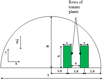
The physical model used in our study is shown in Figure 6.
H=3 m (greenhouse width)
L=6 m (greenhouse length)
e= 0.5 m (plant width)
d= 0.5 m (distandce between rows of plants)
h= 1.2 m (plant height)
Figure 6. Physical model
In order to establish a simple mathematical model that describes the physics of the problem, it is necessary to make a number of simplifying assumptions, namely:
In our study, we will therefore adopt the two-domain approach which consists in writing two systems of equations, one for the fluid medium (Navier-Stokes and energy) and the other for the porous medium (Navier Stokes including the term of Darcy-Brinkman and energy). Taking into account the assumptions made previously, the systems of equations governing our problem is:
3.1 Dimensional equations
Continuity equation:
$\frac{\partial u}{\partial x}+\frac{\partial v}{\partial y}=0$ (1)
- Momentum equation along the x axis:
$\rho_{\mathrm{f}}\left(\mathrm{u} \frac{\partial \mathrm{u}}{\partial \mathrm{x}}+\mathrm{v} \frac{\partial \mathrm{u}}{\partial \mathrm{y}}\right)=-\frac{\partial \mathrm{p}}{\partial \mathrm{x}} \mu_{\mathrm{f}}\left(\frac{\partial^{2} \mathrm{u}}{\partial \mathrm{x}^{2}}+\frac{\partial^{2} \mathrm{u}}{\partial \mathrm{y}^{2}}\right)$ (2)
- Momentum equation along the y axis:
$\rho_{\mathrm{f}}\left(\mathrm{u} \frac{\partial \mathrm{v}}{\partial \mathrm{x}}+\mathrm{v} \frac{\partial \mathrm{v}}{\partial \mathrm{y}}\right)=-\frac{\partial \mathrm{p}}{\partial \mathrm{y}}+\mu_{\mathrm{f}}\left(\frac{\partial^{2} \mathrm{v}}{\partial \mathrm{x}^{2}}+\frac{\partial^{2} \mathrm{v}}{\partial \mathrm{y}^{2}}\right)+\mathrm{g} \beta_{\mathrm{f}}\left(\mathrm{T}-\mathrm{T}_{0}\right)$ (3)
- Energy equation:
$u \frac{\partial \mathrm{T}}{\partial \mathrm{x}}+v \frac{\partial \mathrm{T}}{\partial \mathrm{y}}=\frac{\lambda_{\mathrm{f}}}{(\rho \mathrm{Cp})_{\mathrm{f}}}\left(\frac{\partial^{2} \mathrm{~T}}{\partial \mathrm{x}^{2}}+\frac{\partial^{2} \mathrm{~T}}{\partial \mathrm{y}^{2}}\right)$ (4)
We propose to assimilate plants to a porous medium; moreover, the software for solving the fluid dynamics equations that we use takes into account in a standard way the porous medium type approach with the discretization of the Darcy-Brinkman equations.
- Continuity equation:
$\frac{\partial \mathrm{u}}{\partial \mathrm{x}}+\frac{\partial \mathrm{v}}{\partial \mathrm{y}}=0$
- Momentum equation along the x axis:
$\frac{\rho_{\mathrm{f}}}{\varepsilon^{2}}\left(\mathrm{u} \frac{\partial \mathrm{u}}{\partial \mathrm{x}}+\mathrm{v} \frac{\partial \mathrm{u}}{\partial \mathrm{y}}\right)=-\frac{\partial \mathrm{p}}{\partial \mathrm{x}}+\mu_{\mathrm{eff}} \nabla^{2} \mathrm{u}-\frac{\mu}{\mathrm{K}} \mathrm{u}$ (5)
- Momentum equation along the y axis:
$\frac{\rho_{\mathrm{f}}}{\varepsilon^{2}}\left(\mathrm{u} \frac{\partial \mathrm{v}}{\partial \mathrm{x}}+\mathrm{v} \frac{\partial \mathrm{v}}{\partial \mathrm{y}}\right)=-\frac{\partial \mathrm{p}}{\partial \mathrm{y}}+\mu_{\mathrm{eff}} \nabla^{2} \mathrm{v}-\frac{\mu}{\mathrm{K}} \mathrm{v}-\rho \mathrm{g}$ (6)
- Energy equation:
$(\rho C p)_{f}\left(u \frac{\partial T}{\partial x}+v \frac{\partial T}{\partial y}\right)=\lambda_{e f f}\left(\frac{\partial^{2} T}{\partial x^{2}}+\frac{\partial^{2} T}{\partial y^{2}}\right)$ (7)
3.2 Dimensionless equations
The dimensionless form is used in order to find general solutions to physical problems independent of measurement systems. It also allows the simplification of the solution of the systems of equations and the reduction of the physical parameters, so our system of equations is made dimensionless by introducing the following dimensionless variables:
$(\mathrm{X}, \mathrm{Y})=\frac{(\mathrm{x}, \mathrm{y})}{\mathrm{L}} ;(\mathrm{U}, \mathrm{V})=\frac{\mathrm{L}}{\alpha_{\mathrm{f}}}(\mathrm{u}, \mathrm{v}) ; \theta=\frac{\mathrm{T}-\mathrm{T}_{0}}{\Delta \mathrm{T}} ; \mathrm{P}=\frac{\mathrm{pL}^{2}}{\rho_{\mathrm{f}} \alpha_{\mathrm{f}}^{2}}$
- Continuity equation:
$\frac{\partial \mathrm{U}}{\partial \mathrm{X}}+\frac{\partial \mathrm{V}}{\partial \mathrm{Y}}=0$
- Momentum equation along the X axis:
$\rho_{\mathrm{f}}\left(\mathrm{U} \frac{\partial \mathrm{U}}{\partial \mathrm{X}}+\mathrm{V} \frac{\partial \mathrm{U}}{\partial \mathrm{Y}}\right)=-\frac{\partial \mathrm{P}}{\partial \mathrm{X}}+\operatorname{Pr}\left(\frac{\partial^{2} \mathrm{U}}{\partial \mathrm{X}^{2}}+\frac{\partial^{2} \mathrm{U}}{\partial \mathrm{Y}^{2}}\right)$ (8)
- Momentum equation along the Y axis:
$\rho_{\mathrm{f}}\left(\mathrm{U} \frac{\partial \mathrm{V}}{\partial \mathrm{X}}+\mathrm{V} \frac{\partial \mathrm{V}}{\partial \mathrm{Y}}\right)=-\frac{\partial \mathrm{P}}{\partial \mathrm{Y}}+\operatorname{Pr}\left(\frac{\partial^{2} \mathrm{~V}}{\partial \mathrm{X}^{2}}+\frac{\partial^{2} \mathrm{~V}}{\partial \mathrm{Y}^{2}}\right)+\operatorname{RaPr} \theta$ (9)
- Energy equation:
$\mathrm{U} \frac{\partial \theta}{\partial \mathrm{X}}+\mathrm{V} \frac{\partial \theta}{\partial \mathrm{Y}}=\frac{\partial^{2} \theta}{\partial \mathrm{X}^{2}}+\frac{\partial^{2} \theta}{\partial \mathrm{Y}^{2}}$ (10)
- Continuity equation:
$\frac{\partial \mathrm{U}}{\partial \mathrm{X}}+\frac{\partial \mathrm{V}}{\partial \mathrm{Y}}=0$
- Momentum equation along the X axis:
$\frac{1}{\varepsilon^{2}}\left(\mathrm{U} \frac{\partial \mathrm{U}}{\partial \mathrm{X}}+\mathrm{V} \frac{\partial \mathrm{U}}{\partial \mathrm{Y}}\right)=-\frac{\partial \mathrm{P}}{\partial \mathrm{X}}+\mathrm{R} \cdot \operatorname{Pr}\left(\frac{\partial^{2} \mathrm{U}}{\partial \mathrm{X}^{2}}+\frac{\partial^{2} \mathrm{U}}{\partial \mathrm{Y}^{2}}\right)-\frac{\operatorname{Pr}}{\mathrm{Da}} \mathrm{U}+\operatorname{RaPr} \theta$ (11)
- Momentum equation along the Y axis:
$\frac{1}{\varepsilon^{2}}\left(\mathrm{U} \frac{\partial \mathrm{V}}{\partial \mathrm{X}}+\mathrm{V} \frac{\partial \mathrm{V}}{\partial \mathrm{Y}}\right)=-\frac{\partial \mathrm{P}}{\partial \mathrm{Y}}+\mathrm{R} \cdot \operatorname{Pr}\left(\frac{\partial^{2} \mathrm{~V}}{\partial \mathrm{X}^{2}}+\frac{\partial^{2} \mathrm{~V}}{\partial \mathrm{Y}^{2}}\right)-\frac{\mathrm{Pr}}{\mathrm{Da}} \mathrm{V}+\mathrm{RaPr} \theta$ (12)
- Energy equation:
$\mathrm{U} \frac{\partial \theta}{\partial \mathrm{X}}+\mathrm{V} \frac{\partial \theta}{\partial \mathrm{Y}}=\lambda_{\mathrm{r}}\left(\frac{\partial^{2} \theta}{\partial \mathrm{X}^{2}}+\frac{\partial^{2} \theta}{\partial \mathrm{Y}^{2}}\right)$ (13)
The dimensionless parameters characterizing our problem are:
$\operatorname{Pr}=\frac{v_{\mathrm{f}}}{\alpha_{\mathrm{f}}} ; \mathrm{Ra}=\frac{\mathrm{g} \beta \mathrm{L}^{3} \Delta \mathrm{T}}{v_{\mathrm{f}} \alpha_{\mathrm{f}}} ; \mathrm{Da}=\frac{\mathrm{K}}{\mathrm{L}^{2}} ; \lambda_{\mathrm{r}}=\frac{\lambda_{\mathrm{m}}}{\lambda_{\mathrm{f}}} ; \mathrm{R}=\frac{\mu_{\mathrm{eff}}}{\mu_{\mathrm{f}}}$
Table 1 includes the hydrodynamic and thermal boundary conditions used in this study and which correspond to the climatic conditions of the Adrar region in winter.
Table 1. Boundary conditions
|
Wall |
Velocity |
Temperature |
|
Superior (blanket) |
u=v=0 |
q=0 |
|
Lower (ground) |
u=v=0 |
q=1 |
|
Fluid / Plant interface |
Continuity |
Continuity |
In order to solve the system of partial differential Eqns. (1), (8)-(10) in fluid medium and (1), (11)-(13) in porous medium, we used the Galerkin solution method. We tried several meshes and we opted for a mesh comprising 5600 elements. Figure 7 represents the mesh used and which is a linear triangular mesh.
Figure 7. Adopted mesh
The results from the numerical simulation of natural convection in the greenhouse which is the subject of this study are presented in order to determine the flow and heat transfer within the greenhouse.
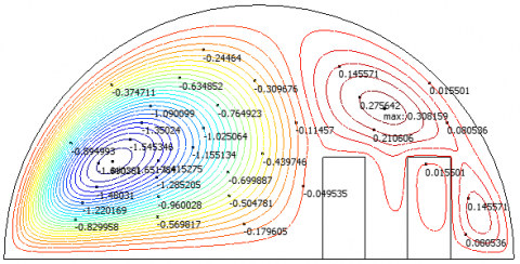
4.1 Isotherms and streamlines
Figures 8 and 9 represent the streamlines (below) and the isotherms (above) for a Darcy number Da = 0.002, a porosity $\varepsilon$ = 0.531 and for different values of the Rayleigh number. For low values of the Rayleigh number (Ra=103 and Ra=104), the isotherms represent lines parallel to each other thus promoting heat transfer by conduction. There is hardly any movement of the air either far or near the plant. For the other values of the Rayleigh number (Ra=105 and Ra=106), the air flow becomes intense as the latter increases giving rise to heat transfer by convection in the greenhouse.
Whatever the value of Rayleigh number, the structure of the streamlines is characterized by two main counter-rotating cells, the one on the right is located above the plant. By increasing the value of Rayleigh number, this cell widens to the detriment of the one on the left. Air circulation around the two rows of plants increases. This circulation gives freshness to the plant promoting the triggering of biochemical processes.
(a)
(b)
Figure 8. Isotherms and streamlines for Da=0.002; $\varepsilon$=0.531 (a) Ra=103 – (b) Ra=104
(a)
(b)
Figure 9. Isotherms and streamlines for Da=0.002; $\varepsilon$=0.531 (a) Ra=105 – (b) Ra=106
4.2 Temperature evolution
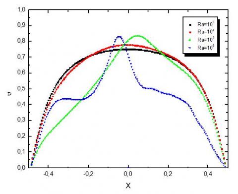
The Figure 10 represents the variation of temperature along the horizontal of the greenhouse passing through the mid-height of the plant (Y=0.1).
For low values of the Rayleigh number (Ra=103 and Ra=104), the shape of the curve is the same, noting a maximum at the level of the axis of symmetry (X=0). These low Rayleigh number values have little influence on the temperature distribution within the greenhouse. For the other values of the Rayleigh number (Ra=105 and Ra=106), both curves have an extremum (maximum). The maximum temperature is little influenced by the value of the Rayleigh number. The axis of symmetry of these curves coincides with the axis of symmetry of the greenhouse. The curve loses its symmetry as Rayleigh number decreases.
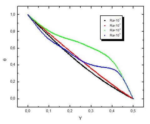
The Figure 11 represents the evolution of the temperature along the median which presents the axis of symmetry of the greenhouse (X = 0). Whatever the value of Ra, the temperature decreases going from the bottom (ground) to the top (roof). For low values of Rayleigh number (Ra=103 and Ra=104), the decrease in temperature is almost linear. It loses its linearity for the other values of Rayleigh number (Ra=105 and Ra=106).
Figure 10. $\theta$ vs X for Y=0.1; Da=0.002; $\varepsilon$=0.531
This decrease in temperature from bottom to top gives a warmer environment below the leaves of the plant than the top giving a favorable climate for the growth of the tomato plant.
The Figure 12 represents the temperature evolution along the vertical passing through the middle between the two rows of plants where the temperature sensor has been placed.
Figure 11. $\theta$ vs Y for X=0; Da=0.002; $\varepsilon$=0.531
Figure 12. $\theta$ vs Y for X=0.25; Da=0.002; $\varepsilon$=0.531
4.3 Velocity Field and stream function
Figure 13 shows the evolution of the vertical component of the velocity along the vertical representing the line of symmetry of the greenhouse. For low Rayleigh number values, the velocity is almost zero, thus promoting conduction. For other Rayleigh number values, the velocity increases with increasing of Rayleigh number. The velocity is maximum at half height of the greenhouse.
Figure 13. V vs Y for X=0; Da=0.002; $\varepsilon$=0.531
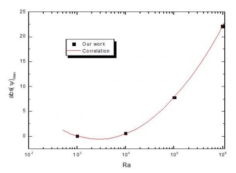
Figure 14 shows the variation of the maximum current function as a function of the number of Ra. She believes in a parabolic way. This growth is represented by the correlation given by Eq. (14) with a square of the correlation coefficient R2 is of the order of unity.
Figure 14. abs($\psi$)max vs Ra For Da=0.002; $\varepsilon$=0.531
${{a b s}}(\psi)_{\max }=a \cdot R a^{2}+b \cdot R a+c$ (14)
a, b and c represent constants, with:
a=3.44; b= -23.64; c=40.03; R2=0.99998
The greenhouse which is the subject of this study is located in the region of Adrar in southwest Algeria. This greenhouse is intended for experimentation in the agricultural field.
In this work, we conducted two types of research:
1- On the one hand, the experimental part of this work focuses on determining the climatic parameters favorable to the growth of the plant and more particularly to that of the tomato plant. For this reason, we have placed sensors to measure the temperature and humidity inside the greenhouse.
2- On the other hand, the theoretical part relates to the numerical resolution by the finite element method of the system of partial differential equations governing the phenomenon of heat transfer and the flow of air within the said greenhouse. The results found show that, for low values of the Rayleigh number, the heat transfer is almost conductive, which takes place at the level of the plant, thus heating the constituents of the latter. While for large Rayleigh numbers, heat transfer by convection becomes dominant which increases the intensity of the air flow and causes it to circulate even around the plant.
In conclusion, to have a favorable environment for the growth of tomatoes, we must keep the openings closed especially during the night without needing a heating system, especially in this region characterized by a hyper arid climate. The value of the temperature calculated by numerical simulation at the position where the sensor has been placed will be compared with that measured by the sensor and which is the subject of another work which will be the continuity of this one followed by a study during the summer period.
We gratefully acknowledge the General Directorate of Scientific Research and Technological Development (DGRSDT) for its financial support and unwavering encouragement.
|
Cp |
Specific heat, J. kg-1. K-1 |
|
Da |
Darcy number |
|
g |
gravitational acceleration, m.s-2 |
|
d |
distance between rows of plants, m |
|
e |
plant width, m |
|
h |
plant height m |
|
H |
greenhouse height, m |
|
K |
Permeability, m-2 |
|
L |
Greenhouse width, m |
|
p |
Dimensional pression, N.m-2 |
|
P |
Dimensionless pression |
|
Pr |
Prandlt number |
|
R |
Dynamic viscosity ratio, R=meff/mf |
|
Ra |
Rayleigh number |
|
T |
Dimensional temperature, ℃ |
|
u,v |
Dimensional Components velocity, m.s-1 |
|
U,V |
Dimensionless Components velocity |
|
x,y |
Dimensional coordinates, m |
|
X,Y |
Dimensionless coordinates |
|
Greek symbols |
|
|
a |
thermal diffusivity, m2. s-1 |
|
b |
thermal expansion coefficient, K-1 |
|
µ |
Dynamic viscosity, kg. m-1.s-1 |
|
e |
Porosity |
|
q |
Dimensionless temperature |
|
r |
Density, kg.m-3 |
|
l |
Thermal conductivity, W.m-1. K-1 |
|
Indices |
|
|
f |
fluid |
|
eff |
effective |
|
m |
matrix |
[1] Haxaire, R. (1999). Caracterisation and modeling of air flow in a greenhouse. Ph D thesis, Faculte des Sciences, Universite de Nice Sophie Antipolis, France, pp. 1-148.
[2] Boulard, T., Haxaire, R., Lamrani, M.A., Roy, J.C., Jaffrin, A. (1999). Characterization and modeling of the air fluxes induced by natural ventilation in a greenhouse. Journal of Agricultural Engineering Research, 74(2): 135-144.
[3] Draoui, B., Benyamine, M., Touhami, Y., Tahri, B. (1999). Numerical simulation of natural convection in transient laminar regime in a bottom heated tunnel greenhouse (Flux). Journal of Renewable Energies, 141-145. https://www.cder.dz/vlib/revue/nspeciauxpdf/jnv_28.pdf.
[4] Wang, S., Boulard, T., Haxaire, R. (1999). Air speed profiles in a naturally ventilated greenhouse with a tomato crop. Agricultural and Forest Meteorology, 96: 181-188.
[5] Ould Khaoua, S.A., Bournet, P.E., Migeon, C., Chassériaux, G., Boulard, T. (2006). Analysis of greenhouse ventilation efficiency with CFD. Bio-Sys Engineering, 95(1): 83-98. https://doi.org/10.1016/j.biosystemseng.2006.05.004
[6] Bougoul, S., Zeroual, S., Boulard, T., Azil, F. (2007). Numerical simulation of air movement and temperature variation in heated greenhouses. Journal of Renewable Energies, 209-212, CER’07, Oujda, Morroco. https://www.cder.dz/download/cer07_47.pdf.
[7] Baxevanou, C., Fidaros, D., Bartzanas, T., Kittas, C. (2010). Numerical simulation of solar radiation, air flow and temperature distribution in a naturally ventilated tunnel greenhouse. Agric. Eng. Int.: CIGR Journal, 12(3): 48-67.
[8] Bartzanas, T., Kittas, C., Tadj, N., Draoui, B. (2007). Influence of vents type arrangement on greenhouse thermal driven ventilation. 2nd PALENC Conference and 28th AIVC Conference on Building Low Energy Cooling and 111 Advanced Ventilation Technologies in the 21st Century, Crete Island, Greece. https://www.aivc.org/sites/default/files/members_area/medias/pdf/Conf/2007/PalencAIVC2007_ 023.pdf.
[9] Kruger, S., Pretorius, L. (2016). Heat transfer in two and three-dimensional single span greenhouses. 10th South African Conference on Computational and Applied Mechanics.
[10] Elashmawy, M., Al-Rashed, A.A.A.A., Kolsi, L., Badawy, I.A.Q., Ali, N.B., Ali, S.S. (2017). Heat transfer and fluid flow in naturally ventilated greenhouses. Engineering, Technology & Applied Science Research, 7(4): 1850-1854. https://doi.org/10.48084/etasr.1269
[11] Mesmoudi, K., Meguellati, K., Bournet, P.E. (2017). Thermal analysis of greenhouses installed under semi-arid climate. International Journal of Heat and Technology. 35(3): 474-486. https://doi.org/10.18280/ijht.350304
[12] Shivayogi Swamy, K.M., Praveen Kumar, M., Santosh Kumar, K. (2017). Numerical analysis of airflow and temperature distribution in a naturally ventilated greenhouse. Journal of Research in Science, Technology, Engineering and Management, 79-86.
[13] Raza, S.S., El Kadi, K., Janajreh, I. (2018). Greenhouse microclimate flow simulation: influence of inlet flow conditions. Int. J. of Thermal & Environmental Engineering, 17(1): 11-18. https://doi.org/10.5383/ijtee.17.01.002
[14] Ouarhlent, F., Soudani, A. (2019). Numerical study of thermal convection in a porous medium. Instrumentation Mesure Metrologie, 18(1): 69-74. https://doi.org/10.18280/i2m.180111
[15] Ghani, S., El-Bialy, E.M.A.A., Bakochristou, F., Rashwan, M.M., Abdelhalim, A.M., Ismail, S.M., Ben, P. (2020). Experimental and numerical investigation of the thermal performance of evaporative cooled greenhouses in hot and arid climates. Science and Technology for the Built Environment, 26(2): 141-160. https://doi.org/10.1080/23744731.2019.1634421
[16] Ghernaout, B., Attia, M.E., Bouabdallah, S., Driss, Z., Benali, M.L. (2020). Heat and fluid flow in an agricultural greenhouse. International Journal of Heat and Technology, 38(1): 92-98. https://doi.org/10.18280/ijht.380110
[17] Jehhef, K.A., Khdair, M.A.S., Thajeel, K.J. (2020). Numerical modeling of thermal radiation heat transfers in agricultural greenhouse. The Fourth Postgraduate Engineering Conference. IOP Conf. Series: Materials Science and Engineering, 745: 012072. https://doi.org/10.1088/1757-899X/745/1/0120721