Roman Kulchytsky-Zhyhailo | Stanisław J. Matysiak | Dariusz M. Perkowski*
© 2021 IIETA. This article is published by IIETA and is licensed under the CC BY 4.0 license (http://creativecommons.org/licenses/by/4.0/).
OPEN ACCESS
The paper deals with the thermoelastic problem of a multilayered pipe subjected to normal loadings on its inner surface and temperature differences on its internal and external surfaces. Two types of nonhomogeneous pipe materials of pipe are considered: (1) a ring-layered composite composed of two repeated thermoelastic solids with varying thickness and (2) a functionally graded ring layer. The ring-layered pipe with periodic structure is investigated by using the homogenized model with microlocal parameters. A homogenization approach is proposed for the modelling of the FGM pipe. The analysis of obtained circumferential, radial and axial stress is presented in the form of figures and discussed in detail. It was shown that the proposed approach to the homogenization allows us to correctly calculate the averaged characteristics in the representative cell (the macro-characteristics) and also the characteristics dependent on the choice of the component in the representative cell (the micro-characteristics) for both microperiodic composites and functionally graded materials.
temperature, displacement, thermal stress, composite material, functionally graded material, nonhomogeneous pipe
The development of engineering structures and their applications in various industries require modern materials. The results in the formation of these solids are to be applicable in specific engineering branches. One of such materials is functionally graded materials (FGM). The FGM are characterized by the continuous or step changing mechanical, thermal and chemical properties [1]. Taking into account the chemical and physical properties, changes in the FGM materials can be divided into two groups [2]: a change in chemical composition gradation, a change in the structure or a change in porosity. Functionally graded materials are used as thermal barrier coatings [3] or as wear reduction layers.
A comprehensive review of various ceramic materials applied as thermal barriers is presented by Lee et al. [4]. The thermomechanical properties of the FGM materials used for thermal barriers are discussed by Wang et al. [5], and Chen and Tong [6].
In the literature, many works deal with stress states under the influence of temperature fields for various types of considered bodies, e.g., an empty cylinder [7], plates [8] or a sphere [9, 10]. For the analysis of such problems, the methods used methods should allow to determine distributions of temperature, displacement, heat flux and stress with sufficiently high accuracy.
The three-dimensional problem of thermomechanical deformation of a freely supported rectangular plate subjected to a sudden temperature pulse is analyzed by Vel and Batra [11]. The material of the plate is assumed to be characterized by thermomechanical properties in the form of power-type functions. A cylinder with FGM material is considered [12]. The optimal values of the circumferential stress component are shown to correspond to the shear modulus given in the form of a linear function.
The basis for the analysis of thermoelastic temperature, temperature and stress is the prior determination of a solution to the problem of heat conduction for a solid with functionally graded properties. The papers [13-15] are devoted to the axisymmetrical heat condition problems in the case of the assumption that the heat conductivity coefficient is described by an exponential or power functions of the radius.
The functional gradation of the materials leads to partial differential equations with variable coefficients. Solving such problems within the classical approach is rather difficult. One of the simplification methods relies on approximate averaging techniques. For example, in the paper [16], the approach related to the replacement of bodies with functionally graded properties by a heterogeneous solids consisting of a package of layers, in which the thermomechanical properties of sublayers are averaged and constants, is applied. However, in this case the solution of an approximate system of equations should fulfill the conditions of perfect thermal and mechanical contact on the interfaces and the assumed boundary conditions.
Another approach to the problems of periodic body heat condition is a use of the homogenized model with microlocal parameters [17-19] or the application of the tolerance model [20, 21]. The homogenized model with microlocal parameters is widely used to solve a number of problems for the composite bodies with periodic structure [22-31].
A wide review of the literature on the thermomechanics of functionally graded bodies can be found by Noda [32]. For example, in the paper [33], an exact solution is presented to the three-dimensional thermoelastic problem of a circular plate subjected to thermal and mechanical loadings. It was assumed there that, apart from the Poisson’s ratio, all the thermal and mechanical material are described by exponential functions of the depth of the boundary surface.
The paper [34] presents an approach to solving two or three-dimensional thermoelasticity problems for materials with functionally graded properties using the boundary element method combined with analytical methods. The authors showed that the proposed manner of solving is more effective than the finite element method.
In this paper, the stress field in the nonhomogeneous pipe subjected to the normal pressures on the inner surface and to a temperature difference on the inner and outer surfaces is investigated. It is assumed that the external pipe surface is unloaded. The pipe is composed of materials with functionally gradation, in which the thermomechanical properties are described by continuous functions of the radius, as well as with the ring layered structures. In the last case, the ideal thermomechanical contact conditions on the interfaces are considered. As a special case, the periodic structure of the pipe material is considered. Certain novel approach to the homogenization with microlocal parameters to modeling of thermoelastic problem of FGM pipe is proposed.
The state of stress in a long nonhomogeneous pipe with the radiuses: internal R0 and external R1 is investigated. The stress field is caused by normal pressures p0 applied to the inner pipe surface and by a temperature difference θ0 in its inner and outer surfaces (see Figure 1). The external pipe surface is unloaded. The considerations will be led using the dimensionless cylindrical coordinates (r, φ, z) related to the dimension R1. It is assumed that the considered problem is axially symmetrical and its solution is independent of the coordinate z in the axial direction. Similarly, as in the classical homogeneous pipe problem [35], it will be assumed that the axial displacement is equal to zero everywhere, but the axial stress is non-zero. In the case of the pipe with unloaded boundaries, the boundary conditions at the ends of the pipe are neglected. Additionally, applying uniform axial stress and taking its value in such manner that the total resultant force in the axial direction is zero, we obtain on both pipe ends the self -balanced distribution of axial pressures. According to the Saint-Venant principle, it causes only local effects near the end of the pipe ends [29]. Since imposing additional uniform axial stress does not cause changes in the distribution of radial and circumferential stress, its influence in the framework of this article will be omitted.
The nonhomogeneous pipe in its cross section is composed of n=2m ring layers (see Figure 1), where m is the number of representative cells. The representative cell with dimensionless thickness δ=(1-r0)/m, (r0=R0/R1) contains two homogeneous ring layers with Young modules E1, E2, Poisson coefficients ν1, ν2, the coefficients of linear thermal expansion α1, α2, the thermal conductivity coefficients K1, K2, and dimensionless thickness δ1=ηδ, δ2=(1-η)δ, where the parameter η$\in$(0,1) describes the contents of the first kind of material and can vary along the thickness of the pipe. The pipe components are located in the regions $r_{i-1}<r<r_{i}, i=1,2, \ldots, n$ respectively, where $r_{2 j}=r_{0}+j \delta, r_{2 j-1}=r_{2 j}-\delta_{2}, j=1,2, \ldots, m.$ The ideal thermal and mechanical contact between the pipe components is taken into account.
Figure 1. The scheme of considered problem
Considering the nonhomogeneous pipe characterized by the mechanical and thermal properties, the fields of displacement, temperature and stress in its i-th, i=1,…,n components will be described using the following state functions: the radial displacement $u^{(i)}$, the radial $\sigma_{r r}^{(i)}$, the circumferential $\sigma_{\varphi \varphi}^{(i)}$ and the axial $\sigma_{z z}^{(i)}$ components of stress tensor $\sigma^{(i)}$ and the temperature $T^{(i)}$. The introduced functions can be calculated by solving the following system of differential equations:
$\frac{d}{d r}\left(r \frac{d T^{(i)}}{d r}\right)=0$ (1a)
$\frac{d}{d r}\left(\frac{1}{r} \frac{d}{d r}\left(r u^{(i)}\right)-\frac{1+v^{(i)}}{1-v^{(i)}} \alpha^{(i)} T^{(i)}\right)=0$; (1b)
$\frac{\sigma_{r r}^{(i)}}{2 \mu^{(i)}}=\frac{1-v^{(i)}}{1-2 v^{(i)}} \frac{d u^{(i)}}{d r}+\frac{v^{(i)}}{1-2 v^{(i)}} \frac{u^{(i)}}{r}-\frac{1+v^{(i)}}{1-v^{(i)}} \alpha^{(i)} T^{(i)}$ (1c)
$\frac{\sigma_{\varphi \varphi}^{(i)}}{2 \mu^{(i)}}=\frac{v^{(i)}}{1-2 v^{(i)}} \frac{d u^{(i)}}{d r}+\frac{1-v^{(i)}}{1-2 v^{(i)}} \frac{u^{(i)}}{r}-\frac{1+v^{(i)}}{1-v^{(i)}} \alpha^{(i)} T^{(i)}$ (1d)
$\sigma_{z z}^{(i)}=v^{(i)}\left(\sigma_{r r}^{(i)}+\sigma_{\varphi \varphi}^{(i)}\right)-E^{(i)} \alpha^{(i)} T^{(i)}$;
$r \in\left(r_{i-1}, r_{i}\right), i=1,2, \ldots, n$ (1e)
and satisfying the boundary conditions on the internal and external surfaces of the pipe:
$\sigma_{r r}^{(1)}\left(r_{0}\right)=-p_{0}, \sigma_{r r}^{(n)}\left(r_{n}\right)=0$ (2a)
$T^{(1)}\left(r_{0}\right)=\theta_{0}, T^{(n)}\left(r_{n}\right)=0$ (2b)
and the conditions of ideal mechanical and thermal contact between the pipe components
$u^{(i)}\left(r_{i}-0\right)=u^{(i+1)}\left(r_{i}+0\right)$,
$\sigma_{r r}^{(i)}\left(r_{i}-0\right)=\sigma_{r r}^{(i+1)}\left(r_{i}+0\right)$,
$i=1,2, \ldots, n-1$ (3a)
$T^{(i)}\left(r_{i}-0\right)=T^{(i+1)}\left(r_{i}+0\right)$,
$K^{(i)} \frac{d T^{(i)}}{d r}\left(r_{i}-0\right)=K^{(i+1)} \frac{d T^{(i+1)}}{d r}\left(r_{i}+0\right)$,
$i=1,2, \ldots, n-1$, (3b)
where, n(2j-1) = n1, n(2j) = n2, a(2j-1) = a1, a(2j) = a2, K(2j-1) = K1, K(2j) = K2, µ(2j-1) = µ1, µ(2j) = µ2, E(2j-1) = E1, E(2j) = E2, j = 1, 2, ..., m are the Poisson’s coefficients, the coefficients of linear thermal expansion, the coefficients of heat conductivity, the Kirchhoff coefficients, and Young modulus of the subsequent pipe components.
Case 1
In the first place, the case in which the parameter η is constant along the pipe thickness will be investigated. The solution of the problem for multilayered pipe with periodic structure will be compared with the solution of the problem of the homogeneous pipe, in which the mechanical and thermal properties will be determined by using the method of homogenization with microlocal parameters [24]. The received boundary value problem has the form:
$\frac{d}{d r}\left(r \frac{d T_{\mathrm{hom}}}{d r}\right)=0, r \in\left(r_{0}, 1\right)$ (4a)
$A_{1} \frac{d^{2} u_{\text {hom }}}{d r^{2}}+\frac{A_{1}}{r} \frac{d u_{\text {hom }}}{d r}-A_{2} \frac{u_{\text {hom }}}{r^{2}}=$
$=\Lambda_{1} \frac{d T_{\text {hom }}}{d r}+\frac{\left(\Lambda_{1}-\Lambda_{2}\right)}{r} T_{\text {hom }}, r \in\left(r_{0}, 1\right)$; (4b)
$\sigma_{r r}^{\text {hom }}\left(r_{0}\right)=-p_{0}, \sigma_{r r}^{\text {hom }}(1)=0$ (5a)
$T_{\text {hom }}\left(r_{0}\right)=\theta_{0}, T_{\text {hom }}(1)=0$. (5b)
The stress state in the homogenized pipe can be calculated using the following equations:
$\sigma_{r r}^{(1)}=\sigma_{r r}^{(2)}=\sigma_{r r}^{\text {hom }}=A_{1} \frac{d u_{\text {hom }}}{d r}+B \frac{u_{\text {hom }}}{r}-\Lambda_{1} T_{\text {hom }}$ (6a)
$\sigma_{\varphi \varphi}^{(j)}=D_{j} \frac{d u_{\text {hom }}}{d r}+E_{j} \frac{u_{\text {hom }}}{r}-F_{j} T_{\text {hom }}, j=1,2$; (6b)
$\sigma_{z z}^{(j)}=G_{j}\left(\sigma_{r r}^{(j)}+\sigma_{\varphi \varphi}^{(j)}\right)-H_{j} T_{\text {hom }}, j=1,2$ (6c)
In the Eqns. (4)-(6) the following notation is introduced: $u_{\text {hom }}, \sigma_{r r}^{\text {hom }}$ and Thom denote the state functions that describe radial displacement, radial stress and temperature, respectively, which are averaged within the periodicity cell; $\sigma_{r r}^{(i)}, \sigma_{\varphi \varphi}^{(i)}, \sigma_{z z}^{(i)}$ are the radial, circumferential and axial stress in the j-th component of the periodicity cell;
$A_{1}=\frac{\left(\lambda_{1}+2 \mu_{1}\right)\left(\lambda_{2}+2 \mu_{2}\right)}{(1-\eta)\left(\lambda_{1}+2 \mu_{1}\right)+\eta\left(\lambda_{2}+2 \mu_{2}\right)}$ (7a)
$A_{2}=A_{1}+\frac{4 \eta(1-\eta)\left(\mu_{1}-\mu_{2}\right)\left(\lambda_{1}+\mu_{1}-\lambda_{2}-\mu_{2}\right)}{(1-\eta)\left(\lambda_{1}+2 \mu_{1}\right)+\eta\left(\lambda_{2}+2 \mu_{2}\right)}$; (7b)
$B=\frac{(1-\eta) \lambda_{2}\left(\lambda_{1}+2 \mu_{1}\right)+\eta \lambda_{1}\left(\lambda_{2}+2 \mu_{2}\right)}{(1-\eta)\left(\lambda_{1}+2 \mu_{1}\right)+\eta\left(\lambda_{2}+2 \mu_{2}\right)}$ (7c)
$\Lambda_{1}=\frac{(1-\eta) \alpha_{2}\left(3 \lambda_{2}+2 \mu_{2}\right)\left(\lambda_{1}+2 \mu_{1}\right)}{(1-\eta)\left(\lambda_{1}+2 \mu_{1}\right)+\eta\left(\lambda_{2}+2 \mu_{2}\right)}+$
$+\frac{\eta \alpha_{1}\left(3 \lambda_{1}+2 \mu_{1}\right)\left(\lambda_{2}+2 \mu_{2}\right)}{(1-\eta)\left(\lambda_{1}+2 \mu_{1}\right)+\eta\left(\lambda_{2}+2 \mu_{2}\right)}$; (7d)
$\Lambda_{2}=\frac{(1-\eta) \alpha_{2}\left(3 \lambda_{2}+2 \mu_{2}\right) \lambda_{1}}{(1-\eta)\left(\lambda_{1}+2 \mu_{1}\right)+\eta\left(\lambda_{2}+2 \mu_{2}\right)} \quad +$
$+\frac{\eta \alpha_{1}\left(3 \lambda_{1}+2 \mu_{1}\right) \lambda_{2}}{(1-\eta)\left(\lambda_{1}+2 \mu_{1}\right)+\eta\left(\lambda_{2}+2 \mu_{2}\right)} \quad +$
$+2\left(\eta \mu_{2}+(1-\eta) \mu_{1}\right) \quad \times$
$\times \frac{\left(\eta \alpha_{1}\left(3 \lambda_{1}+2 \mu_{1}\right)+(1-\eta) \alpha_{2}\left(3 \lambda_{2}+2 \mu_{2}\right)\right)}{(1-\eta)\left(\lambda_{1}+2 \mu_{1}\right)+\eta\left(\lambda_{2}+2 \mu_{2}\right)}$; (7e)
$D_{j}=\frac{\lambda_{j} A_{1}}{\lambda_{j}+2 \mu_{j}} ; E_{j}=\frac{4 \mu_{j}\left(\lambda_{j}+\mu_{j}\right)+\lambda_{j} B}{\lambda_{j}+2 \mu_{j}}, j=1,2$ (7f)
$F_{j}=\frac{2 \alpha_{j}\left(3 \lambda_{j}+2 \mu_{j}\right) \mu_{j}+\lambda_{j} \Lambda_{1}}{\lambda_{j}+2 \mu_{j}}, j=1,2$ (7g)
$G_{j}=\frac{\lambda_{j}}{2\left(\lambda_{j}+\mu_{j}\right)}, H_{j}=\frac{\mu_{j} \alpha_{j}\left(3 \lambda_{j}+2 \mu_{j}\right)}{\lambda_{j}+\mu_{j}}, j=1,2$ (7h)
The constants λj, μj in Eqns. (7) are Lame constants of the j-th, j=1,2, component of the periodicity cell, and
$\lambda_{j}=\frac{E_{j} v_{j}}{\left(1+v_{j}\right)\left(1-2 v_{j}\right)} ; \mu_{j}=\frac{E_{j}}{2\left(1+v_{j}\right)}$ (8)
It should be emphasized that the proposed homogenization method allows us to directly calculate the stress component in each component of the periodicity cell. It is especially important in the case of the circumferential and axial stress that receive jumps on the interfaces between the pipe components. The radial stress is continuous at the interfaces and they are the same, as follows from the Eq. (6a), in both components of the periodicity cell, and they are equal to the averaged radial stress within the periodicity cell. It is easy to verify, that
$B=\eta D_{1}+(1-\eta) D_{2}$,
$A_{2}=\eta E_{1}+(1-\eta) E_{2}$,
$\Lambda_{2}=\eta F_{1}+(1-\eta) F_{2}$. (9)
Therefore, the averaged circumferential stress is given by
$\sigma_{\varphi \varphi}^{\text {hom }}=\eta \sigma_{\varphi \varphi}^{(1)}+(1-\eta) \sigma_{\varphi \varphi}^{(2)}=$
$=B \frac{d u_{\text {hom }}}{d r}+A_{2} \frac{u_{\text {hom }}}{r}-\Lambda_{2} T_{\text {hom }}$ (10)
The analogous dependence takes place in the case of averaged axial stress.
Because the considered boundary problems are linear, the state functions in both approaches can be presented in the form of a sum of two components. The first component describes the solution to the problem of the elasticity theory related to the loading of the internal pipe surface with normal pressure p0. This solution is constructed under assumption that the temperature is equal to zero. The second component of the solution is associated with the calculation of thermal stress caused by the difference in temperature difference on the inner and outer pipe. It enables an independent analysis of each of the mentioned problems.
In the first direct approach, we are integrating the homogeneous equivalent to Eq. (1b). Their general solutions can be written in the form:
$u^{(i)}(r)=\left(1-2 v^{(i)}\right) s_{2 i-1} r-s_{2 i} r^{-1}$,
$r_{i-1} \leq r \leq r_{i}, i=1,2, \ldots, n$. (11)
The radial displacement u(i) generates the stress tensor, which has nonzero components:
$\left(2 \mu^{(i)}\right)^{-1} \sigma_{i r}^{(i)}(r)=s_{2 i-1}+s_{2 i} r^{-2}$,
$r_{i-1} \leq r \leq r_{i}, i=1,2, \ldots, n$; (12a)
$\left(2 \mu^{(i)}\right)^{-1} \sigma_{\varphi \varphi}^{(i)}(r)=s_{2 i-1}-s_{2 i} r^{-2}$,
$r_{i-1} \leq r \leq r_{i}, i=1,2, \ldots, n$; (12b)
$\sigma_{z z}^{(i)}=v^{(i)}\left(\sigma_{r r}^{(i)}+\sigma_{\varphi \varphi}^{(i)}\right)=4 v^{(i)} \mu^{(i)} S_{2 i-1}$,
$r_{i-1} \leq r \leq r_{i}, i=1,2, \ldots, n .$ (12c)
The unknown parameters $s_{i}, i=1,2, \ldots, 2 n$ in the Eqns. (11) and (12) are calculated using the boundary conditions (2a) and (3a). The following system of equations is obtained:
$s_{1}+\frac{s_{2}}{r_{0}^{2}}=-\frac{p_{0}}{2 \mu^{(1)}}$ (13a)
$\left(1-2 v^{(i)}\right) s_{2 i-1} r_{i}-\frac{s_{2 i}}{r_{i}}+$
$-\left(1-2 v^{(i+1)}\right) s_{2 i+1} r_{i}+\frac{s_{2 i+2}}{r_{i}}=0, i=1,2, \ldots, n-1 ;$ (13b)
$s_{2 i-1}+\frac{s_{2 i}}{r_{i}^{2}}-\frac{\mu^{(i+1)}}{\mu^{(i)}} s_{2 i+1}-\frac{\mu^{(i+1)}}{\mu^{(i)} r_{i}^{2}} s_{2 i+2}=0$,
$i=1,2, \ldots, n-1$; (13c)
$S_{2 n-1}+S_{2 n}=0$ (13d)
Substituting the solution of the system of Eqns. (13) into Eqns. (12) the distribution of stress in the nonhomogeneous pipe is obtained.
In the second approach based on the homogenized model the general solution of homogeneous equivalent of Eq. (4b) has the form:
$u_{\text {hom }}(r)=s_{\text {hom }}^{(1)} r^{\gamma}+s_{\text {hom }}^{(2)} r^{-\gamma}, r_{0} \leq r \leq 1$ (14)
where,
$\gamma=\sqrt{A_{2} / A_{1}}$ (15)
The stress components in the j-th component of the periodicity cell are equal to:
$\sigma_{r r}^{(1)}=\sigma_{r r}^{(2)}=\sigma_{r}^{\text {hom }}=\left(A_{1} \gamma+B\right) s_{\text {hom }}^{(1)} r^{\gamma-1}+$
$-\left(A_{1} \gamma-B\right) s_{\text {hom }}^{(2)} r^{-\gamma-1}$; (16a)
$\sigma_{\varphi \varphi}^{(j)}=\left(D_{j} \gamma+E_{j}\right) s_{\text {hom }}^{(1)} r^{\gamma-1}+$
$-\left(D_{j} \gamma-E_{j}\right) s_{\text {hom }}^{(2)} r^{-\gamma-1}, j=1,2$; (16b)
$\sigma_{z z}^{(j)}=G_{j}\left(\sigma_{r r}^{(j)}+\sigma_{\varphi \varphi}^{(j)}\right), j=1,2$ (16c)
From the boundary conditions (5a) the values of constants $s_{\text {hom }}^{(1)}$ and $s_{\text {hom }}^{(2)}$ are obtained:
$s_{\text {hom }}^{(1)}=\frac{-p_{0} r_{0}}{\left(A_{1} \gamma+B\right)\left(r_{0}^{\gamma}-r_{0}^{-\gamma}\right)} \quad$,
$s_{\text {hom }}^{(2)}=\frac{-p_{0} r_{0}}{\left(A_{1} \gamma-B\right)\left(r_{0}^{\gamma}-r_{0}^{-\gamma}\right)} \quad$. (17)
By plugging Eqns. (17) into (16), the radial, circumferential, and axial stress in both components of the periodicity cell are determined.
The general solutions of Eq. (1) described by the nonhomogeneous pipe have the form:
$T^{(i)}(r) / \theta_{0}=\theta^{(i)}(r)=t_{2 i-1}+t_{2 i} \ln \left(r / r_{i}\right)$,
$r_{i-1} \leq r \leq r_{i}, i=1,2, \ldots, n$; (18a)
$u^{(i)}(r)=\left(1-2 v^{(i)}\right) s_{2 i-1} r-\frac{s_{2 i}}{r}+$
$-\frac{1+v^{(i)}}{1-v^{(i)}} \alpha^{(i)} \theta_{0} \frac{1}{r} \int_{r}^{r_{i}} x \theta^{(i)}(x) d x$,
$r_{i-1} \leq r \leq r_{i}, i=1,2, \ldots, n .$ (18b)
The solutions (18) generate the field of stress.
$\frac{\sigma_{r r}^{(i)}(r)}{2 \mu^{(i)}}=s_{2 i-1}+\frac{s_{2 i}}{r^{2}}+$
$+\frac{1+v^{(i)}}{1-v^{(i)}} \alpha^{(i)} \theta_{0} \frac{1}{r^{2}} \int_{r}^{r_{i}} x \theta^{(i)}(x) d x$,
$r_{i-1} \leq r \leq r_{i}, i=1,2, \ldots, n$; (19a)
$\frac{\sigma_{\phi \varphi}^{(i)}(r)}{2 \mu^{(i)}}=s_{2 i-1}-\frac{s_{2 i}}{r^{2}}+$
$-\frac{1+v^{(i)}}{1-v^{(i)}} \alpha^{(i)} \theta_{0} \frac{1}{r^{2}} \int_{r}^{r_{i}} x \theta^{(i)}(x) d x+$
$-\frac{1+v^{(i)}}{1-v^{(i)}} \alpha^{(i)} \theta_{0} \theta^{(i)}(r)$,
$r_{i-1} \leq r \leq r_{i}, i=1,2, \ldots, n$; (19b)
$\frac{\sigma_{z z}^{(i)}(r)}{2 \mu^{(i)}}=2 v^{(i)} s_{2 i-1}-\frac{1+v^{(i)}}{1-v^{(i)}} \alpha^{(i)} \theta_{0} \theta(r)$,
$r_{i-1} \leq r \leq r_{i}, i=1,2, \ldots, n$. (19c)
The unknown parameters si, i = 1, 2, ..., 2n in Eq. (18a) will be determined from the boundary conditions (2b) and (3b). The following system of equations is obtained:
$t_{1}+t_{2} \ln \left(r_{0} / r_{1}\right)=1$ (20a)
$t_{2 i-1}-t_{2 i+1}-t_{2 i+2} \ln \left(r_{i} / r_{i+1}\right)=0, i=1,2, \ldots, n-1$ (20b)
$K^{(i)} t_{2 i}-K^{(i+1)} t_{2 i+2}=0, i=1,2, \ldots, n-1$ (20c)
$t_{2 n-1}=0$ (20d)
Whereas the parameters si, i = 1, 2, ..., 2n in Eqns. (18b) and (19) will be calculated satisfying the boundary conditions (2a) and (3a), leading to the system of equations:
$S_{1}+\frac{S_{2}}{r_{0}^{2}}=-\tilde{t}_{0}$ (21a)
$\left(1-2 v^{(i)}\right) s_{2 i-1} r_{i}-\frac{s_{2 i}}{r_{i}}-\left(1-2 v^{(i+1)}\right) s_{2 i+1} r_{i}+$
$+\frac{s_{2 i+2}}{r_{i}}=-\tilde{t}_{i} r_{i}, i=1,2, \ldots, n-1$; (21b)
$\frac{\mu^{(i)}}{\mu^{(i+1)}} s_{2 i-1}+\frac{\mu^{(i)}}{\mu^{(i+1)}} \frac{s_{2 i}}{r_{i}^{2}}-s_{2 i+1}+$
$-\frac{s_{2 i+2}}{r_{i}^{2}}=\tilde{t}_{i}, i=1,2, \ldots, n-1$; (21c)
$s_{2 n-1}+s_{2 n}=0$ (21d)
where,
$\tilde{t}_{i}=\frac{1+v^{(i+1)}}{1-v^{(i+1)}} \alpha^{(i+1)} \theta_{0} \times$
$\times\left(2 t_{2 i+1} \tilde{r}_{i}-t_{2 i+2}\left(\tilde{r}_{i}+\frac{1}{2} \ln \left(r_{i} / r_{i+1}\right)\right)\right)$,
$i=0,1, \ldots, n-1 ;$ (22a)
$\tilde{r}_{i}=\frac{r_{i+1}^{2}-r_{i}^{2}}{4 r_{i}^{2}}, i=0,1, \ldots, n-1$ (22b)
By first solving the system of Eqns. (20) and next, the system (21), the constants ti, si, i = 1, 2, ..., 2n, will be determined, and after substituting their values into Eqns. (18) and (19), the state of thermal stress in the considered pipe will be found.
In the second alternative approach based on the homogenization method, the Eq. (4a) is integrated. Its general solution has the following form:
$T_{\text {hom }}(r)=t_{\text {hom }}^{(1)}+t_{\text {hom }}^{(2)} \ln (r), r_{0} \leq r \leq 1$ (23)
Next, the general solution of Eq. (4b) is constructed. For this purpose, to the general solution of homogeneous equivalent of equation of (4b), given in Eq. (14), some special solution should be added. The special solution has the form:
$u_{\text {hom }}^{(1)}(r)=s_{\text {hom }}^{(1 t)} r \ln (r)+s_{\text {hom }}^{(2 t)} r, r_{0} \leq r \leq 1$ (24)
where,
$s_{\text {hom }}^{(1 t)}=\frac{\Lambda_{1}-\Lambda_{2}}{A_{1}-A_{2}} t_{\text {hom }}^{(2)}$ (25a)
$s_{\text {hom }}^{(2 t)}=\frac{\Lambda_{1}-\Lambda_{2}}{A_{1}-A_{2}} t_{\text {hom }}^{(1)}+\frac{2 A_{1} \Lambda_{2}-\Lambda_{1}\left(A_{1}+A_{2}\right)}{\left(A_{1}-A_{2}\right)^{2}} t_{\text {hom }}^{(2)}$ (25b)
The components of the stress tensor in the j-th component of the periodicity cell are given by
$\sigma_{r r}^{(1)}=\sigma_{r r}^{(2)}=\sigma_{r r}^{\text {hom }}=$
$=\left(A_{1} \gamma+B\right) s_{\text {hom }}^{(1)} r^{\gamma-1}-\left(A_{1} \gamma-B\right) s_{\text {hom }}^{(2)} r^{-\gamma-1}+$
$\left(A_{1}+B\right) s_{\text {hom }}^{(1 t)} \ln (r)+A_{1}\left(s_{\text {hom }}^{(1 t)}+s_{\text {hom }}^{(2 t)}\right)+$
$+B s_{\text {hom }}^{(2 t)}-\Lambda_{1} T_{\text {hom }}$, (26a)
$\sigma_{\varphi \varphi}^{(j)}=\left(D_{j} \gamma+E_{j}\right) s_{\text {lom }}^{(1)} r^{\gamma-1}-\left(D_{j} \gamma-E_{j}\right) s_{\text {hom }}^{(2)} r^{-\gamma-1}+$
$+\left(D_{j}+E_{j}\right) s_{\text {lom }}^{(1 t)} \ln (r)+D_{j}\left(s_{\text {lom }}^{(1 t)}+s_{\text {hom }}^{(2 t)}\right)+$
$+E_{j} s_{\text {lom }}^{(2 t)}-F_{j} T_{\text {hom }}, j=1,2$, (26b)
$\sigma_{z z}^{(j)}=G_{j}\left(\sigma_{r r}^{(j)}+\sigma_{\varphi \varphi}^{(j)}\right)-H_{j} T_{\text {hom }}, j=1,2$ (26c)
The boundary conditions (5b) are satisfied, if
$t_{\text {hom }}^{(1)}=0, t_{\text {hom }}^{(2)}=\frac{\theta_{0}}{\ln \left(r_{0}\right)}$ (27)
Whereas, using the boundary conditions (5a), the values of constants $s_{\text {hom }}^{(1)}$ and $s_{\text {hom }}^{(2)}$ are obtained:
$s_{\text {hom }}^{(1)}=\frac{S_{\text {hom }}^{(2 t)} r_{0}+S_{\text {hom }}^{(1 t)}\left(r_{0}^{-\gamma}-r_{0}\right)}{\left(A_{1} \gamma+B\right)\left(r_{0}^{\gamma}-r_{0}^{-\gamma}\right)}$,
$s_{\text {hom }}^{(2)}=\frac{S_{\text {hom }}^{(2 t)} r_{0}+S_{\text {hom }}^{(1 t)}\left(r_{0}^{\gamma}-r_{0}\right)}{\left(A_{1} \gamma-B\right)\left(r_{0}^{\gamma}-r_{0}^{-\gamma}\right)}$, (28)
where,
$S_{\text {hom }}^{(1 t)}=A_{1}\left(s_{\text {hom }}^{(1 t)}+s_{\text {hom }}^{(2 t)}\right)+B s_{\text {hom }}^{(2 t)}$,
$S_{\text {hom }}^{(2 t)}=\Lambda_{1} \theta_{0}-\left(A_{1}+B\right) s_{\text {hom }}^{(1 t)} \ln \left(r_{0}\right)$. (29)
Substituting Eqns. (27) and (28) into (23) and (26), the radial, circumferential, and axial stress in every ring layer of the periodicity cell are calculated.
An analysis of the stress state will be derived using the dimensionless stress. The stress caused by the pressures will be related to the parameter p0. Although thermal stress is related to the parameter E*a*$\theta_{0}$, where E* = min(E1,E2), a* = max(a1,a2). The analysis of the received relations shows that if the mathematical model of the pipe is based on the homogenization method, then the stress distribution caused by the pressures depends on five dimensionless parameters: the ratio between the internal and external radiuses of the pipe r0 = R0/R1, the ratio between the Young modulus of the periodicity cell E1/E2, the two Poisson coefficients of the components of the periodicity cell and the parameter η=δ1/δ. The thermal stress is also dependent on the ratio between the coefficients of linear thermal expansion a1/a2. It can be emphasized that within the problem framework of the considered problem the stress does not depend on the ratio between the coefficients of heat conductions K1/K2. However, if the pipe is treated as a nonhomogeneous solid, one should take into account the number of periodicity cells m (or the number of ring layers n) and also, when performing the calculations of the thermal stress, the parameter K1/K2.
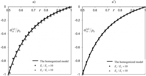
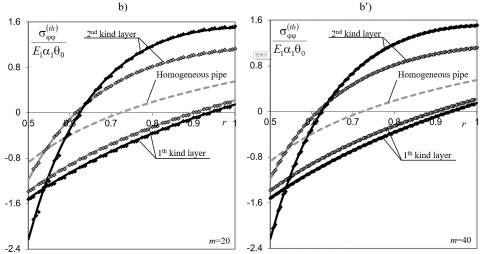
Figure 2. Distribution of radial stress along the pipe thickness; Figure 2a and 2a' are related to the stress caused by normal pressures; Figure 2b and 2b' present the stress caused by the difference in temperature; E1/E2 = 10 (or E2/E1 = 10); 2a for m = 10; 2a' for m = 20; 2b for m = 20; 2b' for m = 40
Figure 3. Distribution of circumferential stress along the pipe thickness; Figure 3a, 3a' are connected with the stress caused by normal pressures; Figure 3b, 3b' present the stress caused by difference of temperature; in Figure 3a, 3a' it is taken E1/E2 = e; in Figure 3b, 3b' it is taken E2/E1 = e; in Figure 3a, 3b it is assumed m = 20; in Figure 3a', 3b' it is assumed m = 40; grey lines and rhombuses are for e = 5; black lines and rhombuses are for e = 10
In order to decrease the number of parameters and decrease the range of their changes, the following assumptions are used:
1) The ratio between the internal and external radiuses of the pipe is 0.5, so r0 = R0/R1 = 0.5;
2) The thickness of each ring layer being the component of pipe is the same, so $\eta$ = 0.5;
3) The Poisson’s ratios both components of periodicity cell are the same and v1 = v2 =0.3;
4) One of the pipe components is a thermal insulator. The applied insulating materials are often characterized by a greater Young modulus but smaller coefficient of linear thermal expansion and smaller coefficient of thermal conductivity. For this reason, the following assumptions, that E1/E2 = a2/a1 = K2/K1 are taken into account;
5) In the aim of an emphasis of possible differences between the solutions obtained by the two presented approaches, some relatively large values of the parameter E1/E2 (or E2/E1) are assumed.
Figure 2 show the distribution of radial stress along the pipe thickness. Figures 2a and 2a' concern the problem, in which the stress is caused by normal pressures p0. Figures 2b and 2b' present the stress distribution caused by differences in temperature on the external and internal pipe surfaces. The continuous lines describe the stress distribution in the pipe obtained within the framework of the homogenization method. Radial stress does not depend on the sequence of ring layers arranged in the periodicity cell. The distribution of radial stress received within the framework of direct approach depends on the sequence of ring layers. The relation is described by using black and grey triangles. The black triangles present the case, when the first component of periodicity cell is the ring layer with larger Young modulus, the grey triangles for the first layer with smaller Young modulus. From Figure 2 it follows that the values of radial stress for the homogenized model are located between the adequate values obtained within the direct approach calculated for the both sequences of insulating ring layers location in the periodicity cell. The difference between the locations of black and grey triangles decreases along with an increase of the number of periodicity cells. The broken lines in Figures 2b and 2b', and in some next figures, describe the stress distribution in the homogeneous pipe with the parameter E* and a*.
The radial stress in the considered problem can be treated as a macro-characteristic, which does not depend on the choice of component of the periodicity cell. The calculations show that the proposed homogenization method allows to calculate, with a good accuracy, not only the macro-characteristics, but also micro-characteristics, which values depend on the choice of the considered component of periodicity cell. An example of such micro-characteristic is the behaviour of the circumferential stress, which is shown in Figure 3. When the homogenization method is applied, there is no information connected with the kind of ring layer in the specified point of pipe. At each point we obtain two equations to calculate the circumferential stress. The equation with the index 1 allows to determine of the circumferential stress in the ring layer of the first kind, and the one with the index 2 - in the ring layer of the second kind. Two continuous lines denoted by numbers 1 and 2 (the indexes of types of layers) are appropriate for the values of circumferential stress in the periodicity cell. In Figure 3 the rhombuses are adequate for the direct approach. If the stress is calculated in the layers with odd numbers, the adequate rhombuses are consistent with the continuous line denoted by 1, in the layers with even numbers, with the continuous line denoted by 2. This means that the continuous lines within the homogenized model correctly determine the distribution of stress in the both ring layers in periodicity cell.
As follows from Figure 3, the highest value of circumferential stress in the elasticity theory problem is taken on the internal pipe surface, but in the case of thermal stress – on the external pipe surface. In both cases, it is the greatest tensile stress. In order to compare the difference calculation of greatest tensile stress, which is caused by an application of both proposed approaches, the sequence of ring layers in the periodicity cell is chosen in such manner, that in the place of appearance of the greatest circumferential stress there is the ring layer with greater Young modulus. For this reason, when calculating the circumferential stress in the problem of elasticity theory, it is assumed that E1/E2 > 1, and in the case of thermal stress we assumed that E2/E1 > 1.
Table 1. Dependence of the tensile stress values on the dimensionless parameter E1/E2 and the number of periodicity cells m
|
|
|
Hom. |
m = 40 |
m = 20 |
m = 10 |
|
$\frac{\max \sigma_{\varphi \varphi}^{(p)}\left(r_{0}\right)}{p_{0}}$ |
E1/E2 = 5 |
3.2954 |
-1.182% |
-2.341% |
-4.590% |
|
$\frac{\max \sigma_{\varphi \varphi}^{(p)}\left(r_{0}\right)}{p_{0}}$ |
E1/E2 = 10 |
4.0037 |
-1.770% |
-3.495% |
-6.804% |
|
$\frac{\max \sigma_{\phi \varphi}^{(t h)}(1)}{E_{1} \alpha_{1} \theta_{0}}$ |
E2/E1 = 5 |
1.1103 |
0.905% |
1.800% |
3.562% |
|
$\frac{\max \sigma_{\varphi \varphi}^{(t h)}(1)}{E_{1} \alpha_{1} \theta_{0}}$ |
E2/E1 = 10 |
1.4982 |
0.897% |
1.763% |
3.405% |
Figure 4. Distribution of axial stress along the pipe thickness; Figure 4a: for the axial stress caused by normal pressures; 4b: for the ones caused by temperature differences; m = 20; 4a for E1/E2 = e; 4b for E2/E1 = e; the grey lines and rhombuses for e = 5; the black lines and rhombuses for e = 10
In the Table 1 the highest values of tensile stress calculated using the homogenization method (column “Hom.”) are given. The relative deviations (given in percent’s) obtained when comparing the values with adequate values received in the direct approach for the numbers of periodicity cells: columns m=40, 20, 10. Based on the results presented in Table 1, it can be concluded that the double increase in layer number caused the double decrease in the difference between the stress analysed. It means, that for the adequate number of cells, the mathematical model of the problem can be based on the homogenization method.
The results analogous to analysed ones are obtained in the case of the axial stress, see Figure 4.
Let the parameter $\eta$ describe the structure of considered nonhomogeneous pipe changes along the pipe thickness (see Figure 5). In the case where every pipe component is considered as an independent thermoelastic body (direct approach), the procedure for solving the problem is the same as in the case of a pipe with periodic structure. As before, Eqns. (1) will be solved and next the boundary conditions (2) and (3) will be used, so the problem will be reduced to solving the linear system algebraic Eqns. (20) and (21).
Figure 5. The scheme of considered problem
Consider the possibility of applying of the relations (6) and (10) to the description of the gradient body. Eqns. (6) and (10) should be supplemented by the relation determining the heat flux in the direction to layering:
$q_{r}=-K_{\mathrm{hom}} \frac{d T_{\mathrm{hom}}}{d r}$ (30a)
where,
$K_{\mathrm{hom}}=\frac{K_{1} K_{2}}{\eta K_{2}+(1-\eta) K_{1}}$ (30b)
Taking into account the dependence of parameter $\eta$ on the variable r, the equation of heat conduction has the form:
$\frac{d}{d r}\left(r K_{\mathrm{hom}}(r) \frac{d T_{\mathrm{hom}}}{d r}\right)=0$ (31)
Substituting the constitutive relations (6a) and (10) into the equilibrium equation of a representative cell.
$\frac{d \sigma_{r r}^{\text {hom }}}{d r}+\frac{\sigma_{r r}^{\text {hom }}-\sigma_{\varphi \varphi}^{\text {hom }}}{r}=0$ (32)
the following differential equation to determine of radial averaged displacement within the representative cell is obtained:
$A_{1} \frac{d^{2} u_{\text {hom }}}{d r^{2}}+\frac{1}{r} \frac{d}{d r}\left(r A_{1}\right) \frac{d u_{\text {hom }}}{d r}-\left(A_{2}-r \frac{d B}{d r}\right) \frac{u_{\text {hom }}}{r^{2}}=$
$=\frac{d\left(\Lambda_{1} T_{\text {hom }}\right)}{d r}+\frac{\left(\Lambda_{1}-\Lambda_{2}\right)}{r} T_{\text {hom }}, r \in\left(r_{0}, 1\right)$. (33)
The boundary conditions still have the form of Eqns. (5).
The solution of differential Eq. (31), which satisfies the boundary conditions (5b) is given in the form:
$\frac{T_{\text {hom }}(r)}{\theta_{0}}=\left(\int_{r_{0}}^{1} \frac{d x}{x K_{\text {hom }}(x)}\right)^{-1}\left(\int_{r}^{1} \frac{d x}{x K_{\text {hom }}(x)}\right)$,
$r_{0} \leq r \leq 1$. (34)
It will be additionally assumed that the function h(r) is the linear function which satisfies the conditions h(r0) = 1, h(r0) = 0:
$\eta(r)=\frac{1-r}{1-r_{0}}, r_{0}<r<1$ (35)
This kind of gradient material is used as a gradient coating to protect of the slowly changing transition from the material properties of substrate to the material properties of the material of external (or internal) insulating coating. For some simplification of the analysis, in this article, the gradient-passing ring layer will be considered independently. The investigations will be limited to the thermal stress, so in the boundary condition (5a) it will be assumed that p0 = 0.
Taking into account the relation (35), the function Thom(r), after integration in the Eq. (34), can be written in the form:
$\frac{T_{\text {hom }}(r)}{\theta_{0}}=\frac{1-r+K_{A} \ln (r)}{1-r_{0}+K_{A} \ln \left(r_{0}\right)}, r_{0} \leq r \leq 1$ (36a)
where,
$K_{A}=\frac{K_{1} r_{0}-K_{2}}{K_{1}-K_{2}}$ (36b)
The differential Eq. (33), which is an equation with changing coefficients, will be solved numerically using the finite difference method. The interval [r0,1] is divided into N equal subintervals. In every internal node the differentials in Eq. (33) are replaced with well-known difference equations based on the nodes. In this manner, we will obtain the equations in the number N-1, which includes (n+1) unknown parameters described the values of the radial displacement ui = uhom($\rho$i) in the nodes $\rho_{i}=r_{0}+i \Delta r$, where $\Delta$r = (1- r0)/N, i = 0, 1, ..., N:
$u_{i-1}-2 u_{i}+u_{i+1}+0.5 a_{i} \Delta r\left(u_{i+1}-u_{i-1}\right)-b_{i}(\Delta r)^{2} u_{i}=$
$=c_{i}(\Delta r)^{2}, i=1,2, \ldots, N-1$, (37)
where,
$a_{i}=\frac{1}{r A_{1}} \frac{d\left(r A_{1}\right)}{d r}, r=\rho_{i}, i=1,2, \ldots, N-1$ (38a)
$b_{i}=\frac{1}{r^{2} A_{1}}\left(A_{2}-r \frac{d B}{d r}\right), r=\rho_{i}, i=1,2, \ldots, N-1$ (38b)
$c_{i}=\frac{1}{A_{1}}\left(\frac{d\left(\Lambda_{1} T_{\text {hom }}\right)}{d r}+\frac{\left(\Lambda_{1}-\Lambda_{2}\right)}{r} T_{\text {hom }}\right)$,
$r=\rho_{i}, i=1,2, \ldots, N-1$. (38c)
The obtained system of equations should be supplemented by two equations obtained by substituting the constitutive relations (6a) into homogenous equivalents of the boundary conditions (5a). In the obtained relations, the differential duhom/dr on the internal ends are replaced by the well-known difference equations based on five nodes
$\Delta r \frac{d u_{\text {hom }}\left(r_{0}\right)}{d r}=-\frac{25}{12} u_{0}+4 u_{1}-3 u_{2}+\frac{4}{3} u_{3}-\frac{1}{4} u_{4}$ (39)
The equation for the differential at the right end r = 1 is obtained from Eq. (39), substituting the parameter $\Delta$r by the parameter -$\Delta$r, and index i (i = 0, 1, 2, 3 and 4) replacing by the index N-i.
The calculations are performed for the parameters N and 2N, selecting the parameter N in such a manner that the difference between obtained approximations of radial displacement does not exceed 0.5%. The calculations show that the required accuracy will be received, if N=40 or N=80 in the dependence on parameters.
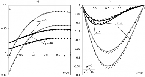
Figure 6. Distribution of dimensionless radial displacement, Figure 6a; and dimensionless radial stress, Figure 6b along the pipe thickness: m = 20; black laines and rhombuses for E1/E2 = e > 1; grey laines and rhombuses for E2/E1 = e > 1
Thermal stress is related to the parameter E*a*q0. The stress state in the homogenized model depends on the six dimensionless parameters: r0, E1/E2, n1, n2, a1/a2 and K1/K2. If the pipe non-homogeneity is taken directly into consideration, number of representative cells m is also an additional parameter. The assumptions presented in Section 5 “Result analysis” beyond assumption 20, which will be replaced by the relation (35) determined the form of function $\eta$(r), are given into consideration.
The distributions of macro-characteristics that is characteristics averaged within the representative cell, are presented. Figure 6a shows the radial displacement along the thickness of the pipe, and Figure 6b presents the radial stress. The distributions of radial displacement and stress in the substitutive gradient pipe, which properties are determined using the homogenization, are given by the continuous lines. The distributions that considered directly the non-homogeneity are presented as rhombuses. One can observe complete qualitative agreement and a very good quantitative agreement of both solutions.
It should be noted that if E1/E2 > 1 (the black lines in Figure 6), the material with thermal properties of the insulator (K1/K2 < 1, as follows from the assumption 4 presented in Section 5 for the choice of the parameters investigated) is on the internal pipe surface. If E1/E2 < 1 (K1/K2 > 1, the grey lines in Figure 6) the insulating properties are on the outer surface of the pipe. That is, that the gradient materials described by the parameters E1/E2 and E2/E1 (E1/E2=E2/E1=e), have fundamentally different thermomechanical properties. For this reason, the black and grey lines (or rhombuses) in Figures 6 differ considerably.
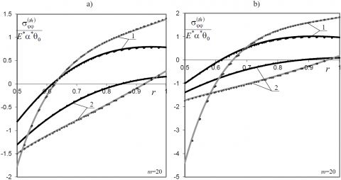
Figures 7 show the distribution of circumferential stress, which in the considered problem depend on the kind of component in the representative cell, so the stress is a micro-characteristics. The lines with number 1 are for the ring layers with a greater Young modulus, and the lines with number 2 for the layers with a smaller Young modulus. As is seen from these figures, the solution of the problem based on the homogenized model also in this case allows one to correctly determine the stress state in every component of the representative cell.
For the determination of quantitative differences between the solutions based on both considered approaches, the Table 2 is presented. In the column “Hom.” in Table 2 the values of circumferential stress on the internal and external pipe surfaces obtained on the basis of homogenization method are presented. It was assumed that in the point r = r0 there is the first ring layer of the representative cell, and in the point r = 1 there is the second layer. In the subsequent columns, the relative deviations (in percent) of these values from the adequate values are obtained considering the number of representative cells m. For the minimization of the influences of numerical errors during the calculations, the values in the column “Hom.”, it was assumed that N=320. Based on the results of calculations from Table 2 it can be concluded that double increase of the cell number causes almost double decrease in the difference between the stress analysed. That is, that also in the case of gradient solids for adequate numbers of cells, the mathematical model can be based on the homogenization method. It can be emphasized that the difference between the solution is greater if E1 > E2 (K1 < K2), so the properties of the insulator are on the internal surface of the pipe.
Figure 7. Distribution of circumferential stress along the pipe thickness: m = 20; the black lines and rhombuses are for E1/E2 = e > 1; the grey lines and rhombuses are for E2/E1 = e > 1; Figure 7a for e = 5; 7b for e = 10; number 1 is adequate for circumferential stress in layers with a higher Young modulus; number 2 is for circumferential stress in layers with a smaller Young modulus
Table 2. Dependence of circumferential stress on the pipe surface on the dimensionless parameter E1/E2 and number of representative cells m
|
|
|
|
“Hom.” |
m = 80 |
m = 40 |
m = 20 |
m = 10 |
|
$\frac{\sigma_{\varphi \varphi}^{(t h)}\left(r_{0}\right)}{E^{*} \alpha^{*} \theta_{0}}$ |
E1 > E2 |
E1/E2 = 5 |
-0.8185 |
-0.393% |
-0.761% |
-1.417% |
-2.467% |
|
E1/E2 = 10 |
-1.0217 |
-1.125% |
-2.192% |
-4.140% |
-7.410% |
||
|
E1 < E2 |
E2/E1 = 5 |
-1.4977 |
0.118% |
0.231% |
0.443% |
0.819% |
|
|
E2/E1 = 10 |
-1.7270 |
0.232% |
0.444% |
0.884% |
1.674% |
||
|
$\frac{\sigma_{\varphi \varphi}^{(t h)}(1)}{E^{*} \alpha^{*} \theta_{0}}$ |
E1 > E2 |
E1/E2 = 5 |
0.1568 |
-0.638% |
-1.262% |
-2.480% |
-4.788% |
|
E1/E2 = 10 |
0.09616 |
-0.915% |
-1.820% |
-3.588% |
-6.957% |
||
|
E1 < E2 |
E2/E1 = 5 |
1.3866 |
0.343% |
0.682% |
1.348% |
2.636% |
|
|
E2/E1 = 10 |
1.8161 |
0.254% |
0.508% |
1.041% |
1.979% |
In the paper, it is shown, that in the framework of the considered problems as well as for the multi-layered pipe with the periodic structure and the multi-layered pipe with gradient structure, the homogenized model can be applied. The proposed approach to homogenization allows us to correctly calculate not only the averaged characteristics in the representative cell (the macro-characteristics) but also the characteristics dependent on the choice of the component in the representative cell (the micro-characteristics). If the pipe has periodic structure, the solution based on the homogenization method takes the form of simple engineering relations. Whereas if the pipe structure is investigated directly in the thermoelastic problem, two systems of linear equations with the dimension 4m, where m is the number of periodicity cell, need to be solved.
When describing the gradient pipe using the homogenization method, one will not obtain an analytical solution. The numerical method was proposed, which leads to a system of 40 – 80 linear algebraic equations. It seems that within the framework of the considered problem, the homogenization method is effective, when the number of representative cells considerably exceeds the number 20. It can be emphasized, that the presented investigations allow to conclude, that the proposed homogenization method can correctly describe the solutions of more complicated problems, in which an independent consideration of representative cell components can be extremely labour-consuming or sometimes simply impossible to accomplish.
The research has been conducted as part of a project at the Faculty of Mechanical Engineering of the Bialystok University of Technology. Project number WZ/WMIIM/3/2020.
|
E |
Young modulus, MPa |
|
K |
thermal conductivity, W.m-1. K-1 |
|
m |
number of the representative cells |
|
n |
number of the ring layers |
|
p0 |
normal pressure applied to the inner pipe surface, MPa |
|
$R_{0}$ |
outer radius of pipe, m |
|
$R_{1}$ |
inner radius of pipe, m |
|
(r, φ, z) |
dimensionless cylinder coordinates related to the inner radius of pipe |
|
T |
temperature deviation in the points of pipe from the temperature of outer medium, K |
|
u |
dimensionless radial displacement related to the inner radius of pipe |
|
Greek symbols |
|
|
$\alpha$ |
coefficient of linear thermal expansion, K-1 |
|
$\delta$ |
dimensionless thickness of representative cells |
|
θ0 |
temperature difference in its inner and outer surface of pipe, K |
|
λ, µ |
Lame’ constants, MPa |
|
µ |
Kircchoff coefficients (the second Lame constant), MPa |
|
v |
Poisson coefficient |
|
σ |
tensor stress, MPa |
|
σrr |
radial components of stress tensor, MPa |
|
σφφ |
circumferential components of stress tensor, MPa |
|
σzz |
axial components of stress tensor, MPa |
[1] Hernik, S. (2016). Wear resistance of piston sleeve made of layered material structure: MMC A356R, anti-abrasion layer and FGM interface. Acta Mechanica et Automatica, 10(3): 207-212. https://doi.org/10.1515/ama-2016-0031.
[2] Masayuki, N., Toshio, H., Ryuzo, W. (1987). Functionally gradient materials. In pursuit of super heat resisting materials for spacecraft. Journal of the Japan Society for Composite Materials, 13(6): 257-264.
[3] Matysiak, S., Perkowski, D. (2016). On heat conduction problems in a composite half-space with a nonhomogeneous coating. Heat Transfer Research, 47(12): 1141-1155. https://doi.org/10.1615/HeatTransRes.2016013425
[4] Lee, W.Y., Stinton, D.P., Berndt, C.C., Erdogan, F., Lee, Y.D., Mutasim, Z. (1996). Concept of functionally graded materials for advanced thermal barrier coating applications. Journal of the American Ceramic Society, 79(12): 3003-3012. https://doi.org/10.1111/j.1151-2916.1996.tb08070.x
[5] Wang, B.L., Han, J.C., Du, S.Y. (2000). Crack problems for functionally graded materials under transient thermal loading. Journal of Thermal Stresses, 23(2): 143-168. https://doi.org/10.1080/014957300280506
[6] Chen, B., Tong, L. (2004). Sensitivity analysis of heat conduction for functionally graded materials. Materials & Design, 25(8): 663-672. https://doi.org/10.1016/j.matdes.2004.03.007
[7] Ootao, Y., Ishihara, M. (2014). Transient thermoelastic analysis for a multilayered hollow cylinder with piecewise power law nonhomogeneity due to asymmetric surface heating. Acta Mechanica, 225(10): 2903-2922. https://doi.org/10.1007/s00707-014-1204-3.
[8] Tanigawa, Y., Ootao, Y., Kawamura, R. (1991). Thermal bending of laminated composite rectangular plates and nonhomogeneous plates due to partial heating. Journal of Thermal Stresses, 14(3): 285-308. https://doi.org/10.1080/01495739108927069
[9] Ootao, Y. (2011). Transient thermoelastic analysis for a multilayered hollow sphere with piecewise power law nonhomogeneity. Composite Structures, 93(7): 1717-1725. https://doi.org/10.1016/j.compstruct.2010.12.008
[10] Kushnir, R.M., Yasinskyy, A.V., Tokovyy, Y.V. (2021). Effect of material properties in the direct and inverse thermomechanical analyses of multilayer functionally graded solids. Advanced Engineering Materials, 2100875. https://doi.org/10.1002/adem.202100875
[11] Vel, S.S., Batra, R.C. (2003). Three-dimensional analysis of transient thermal stresses in functionally graded plates. International Journal of Solids and Structures, 40(25): 7181-7196. https://doi.org/10.1016/S0020-7683(03)00361-5
[12] Batra, R.C. (2008). Optimal design of functionally graded incompressible linear elastic cylinders and spheres. AIAA Journal, 46(8): 2050-2057. https://doi.org/10.2514/1.34937
[13] Ootao, Y., Tanigawa, Y. (2006). Transient thermoelastic analysis for a functionally graded hollow cylinder. Journal of Thermal Stresses, 29(11): 1031-1046. https://doi.org/10.1080/01495730600710356
[14] Sladek, J., Sladek, V., Zhang, C. (2003). Transient heat conduction analysis in functionally graded materials by the meshless local boundary integral equation method. Computational Materials Science, 28(3-4): 494-504. https://doi.org/10.1016/j.commatsci.2003.08.006
[15] Wang, B.L., Mai, Y.W. (2005). Transient one-dimensional heat conduction problems solved by finite element. International Journal of Mechanical Sciences, 47(2): 303-317. https://doi.org/10.1016/j.ijmecsci.2004.11.001
[16] Hosseini, S.M., Akhlaghi, M., Shakeri, M. (2008). Heat conduction and heat wave propagation in functionally graded thick hollow cylinder base on coupled thermoelasticity without energy dissipation. Heat and Mass Transfer, 44(12): 1477-1484. https://doi.org/10.1007/s00231-008-0381-9
[17] Matysiak, S.J., Woźniak, C. (1987). On the modelling of heat conduction problem in laminated bodies. Acta Mechanica, 65(1): 223-238. https://doi.org/10.1007/BF01176884
[18] Matysiak, S. (1991). On certain problems of heat conduction in periodic composites. ZAMM‐Journal of Applied Mathematics and Mechanics/Zeitschrift für Angewandte Mathematik und Mechanik, 71(12): 524-528. https://doi.org/10.1002/zamm.19910711218
[19] Matysiak, S.J., Perkowski, D.M. (2014). Temperature distributions in a periodically stratified layer with slant lamination. Heat and Mass Transfer, 50(1): 75-83. https://doi.org/10.1007/s00231-013-1225-9
[20] Woźniak, C., Wierzbicki, E. (2000). Averaging techniques in thermomechanics of composite solids: Tolerance Averaging versus Homogenization. Wydawn. politechniki Częstochowskiej.
[21] Woźniak, C., Michalak, B., Jędrysiak, J., Matysiak, S., Świtka, R. (2008). Thermomechanics of microheterogeneous solids and structures: Tolerance averaging approach. Wydawnictwo Politechniki Łódzkiej.
[22] Matysiak, S.J., Perkowski, D.M. (2010). On heat conduction in a semi-infinite laminated layer. Comparative results for two approaches. International Communications in Heat and Mass Transfer, 37(4): 343-349. https://doi.org/10.1016/j.icheatmasstransfer.2009.12.009
[23] Perkowski, D.M., Kulchytsky-Zhyhailo, R., Kołodziejczyk, W. (2018). On axisymmetric heat conduction problem for multilayer graded coated half-space. Journal of Theoretical and Applied Mechanics, 56(1): 147-156. https://doi.org/10.15632/jtam-pl.56.1.147
[24] Kulchytsky-Zhyhailo, R., Matysiak, S.J., Perkowski, D.M. (2011). Plane contact problems with frictional heating for a vertically layered half-space. International Journal of Heat and Mass Transfer, 54(9-10): 1805-1813. https://doi.org/10.1016/j.ijheatmasstransfer.2010.10.040
[25] Matysiak, S.J., Perkowski, D.M. (2011). Axially symmetric problems of heat conduction in a periodically laminated layer with vertical cylindrical hole. International Communications in Heat and Mass Transfer, 38(4): 410-417. https://doi.org/10.1016/j.icheatmasstransfer.2010.12.018
[26] Kulchytsky-Zhyhailo, R., Matysiak, S.J. (2005). On heat conduction problem in a semi-infinite periodically laminated layer. International Communications in Heat and Mass Transfer, 32(1-2): 123-132. https://doi.org/10.1016/j.icheatmasstransfer.2004.08.023
[27] Kaczyński, A., Matysiak, S.J. (1988). On the complex potentials of the linear thermoelasticity with microlocal parameters. Acta Mechanica, 72(3): 245-259. https://doi.org/10.1007/BF01178311
[28] Kulchytsky-Zhyhailo, R., Matysiak, S.J., Perkowski, D.M. (2020). On the quasi-stationary problem of heat conduction for a homogeneous half-space with composite coating. Acta Mechanica, 231(3): 1241-1251. https://doi.org/10.1007/s00707-019-02591-9
[29] Kulchytskyy, R., Matysiak, S.J., Perkowski, D.M. (2021). Heat conduction problems in a homogeneous pipe with inner nonhomogeneous coating. International Journal of Heat and Technology, 39(1): 23-31. https://doi.org/10.18280/ijht.390103
[30] Sebestianiuk, P., Perkowski, D.M., Kulchytsky-Zhyhailo, R. (2020). On contact problem for the microperiodic composite half-plane with slant layering. International Journal of Mechanical Sciences, 182: 105734. https://doi.org/10.1016/j.ijmecsci.2020.105734
[31] Sebestianiuk, P., Perkowski, D.M., Kulchytsky-Zhyhailo, R. (2019). On stress analysis of load for microperiodic composite half-plane with slant lamination. Meccanica, 54(3): 573-593. https://doi.org/10.1007/s11012-019-00970-z
[32] Noda, N. (1999). Thermal stresses in functionally graded materials. Journal of Thermal Stresses, 22(4-5): 477-512. https://doi.org/10.1080/014957399280841
[33] Jabbari, M., Shahryari, E., Haghighat, H., Eslami, M.R. (2014). An analytical solution for steady state three dimensional thermoelasticity of functionally graded circular plates due to axisymmetric loads. European Journal of Mechanics-A/Solids, 47: 124-142. https://doi.org/10.1016/j.euromechsol.2014.02.017
[34] Yang, K., Feng, W.Z., Peng, H.F., Lv, J. (2015). A new analytical approach of functionally graded material structures for thermal stress BEM analysis. International Communications in Heat and Mass Transfer, 62: 26-32. https://doi.org/10.1016/j.icheatmasstransfer.2015.01.009
[35] Timoshenko, S.P., Goodier, J.N. (1961). Theory of Elasticity. McGraw-Hill.