Leonard Ribot Chuisseu Nguewo* | Marcel Brice Obounou Akong | Clement Tchawoua | Prosper Gopdjim Noumo | Fabrice Mbakop Kwefeu | Noel Djongyang
© 2021 IIETA. This article is published by IIETA and is licensed under the CC BY 4.0 license (http://creativecommons.org/licenses/by/4.0/).
OPEN ACCESS
Thermo PhotoVoltaic (TPV) system convert into electrical energy the radiation emitted from an artificial heat source (i.e., solar or combustion) by the use of photovoltaic cells. In the last decade, TPV system has gained an increasing attention as cogeneration system for the distributed generation sector. Nevertheless, these systems are not fully developed and studied: several aspects need to be further investigated and completely understood. In this study, we modeled and investigated by performing numerical simulation on the feasibility of the TPV system exploiting waste heat energy during biomass combustion. To achieve this goal, we considered a TPV system in which we evaluated and analyzed the waste heat flux resulting from the combustion of the palm nuts shells as well as the corresponding temperature received at the surface of the TPV Thermal-emitter. Furthermore, we evaluated the heat intensity. Results obtained shows that the average temperature at the TPV absorber-emitter is around 1600k. Different variation of the net heat flux at the TPV absorber-emitter are observed for different position. The maximum heat intensity is around 15*1010 W.m-2.µm-1 for a wave length of 2000 nm. These results indicate that the model presented herein is therefore suitable for the design of the TPV system.
thermo photovoltaic, combustion, biomass, heat transfer, numerical simulation
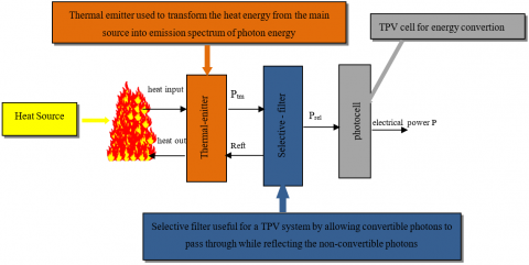
The origins of TPV date back to the early 1960s, but it is only in relatively recent years that it has shown real promise. Incident and output power densities are much larger than flat-plate PhotoVoltaic (PV) modules because of geometric considerations. Potential attractions of TPV include: high power density, fuel versatility, portability, silent operation, operation that is independent of the sun, and low maintenance. Possible applications include: stand-alone domestic gas-furnaces, cogeneration of electricity and heat, large-scale recovery of high-temperature waste heat from industrial processes such as glass-manufacture, and many others [1]. The concept of TPV system is to convert thermal energy from a heat source (sun or combustion reaction) directly into electrical energy by means of emitter, filter and photocells [2]. TPV system is composed of four component which are heat source, thermal emitter, spectral filter and arrays of infrared sensitive photovoltaic cells as it is shown in the Figure 1 [3].
From the Figure 1, the heat source can provide from solar radiation or combustion or industrial waste heat [4]; the emitter control the spectral thermal radiation and the filter plays the role of recycling thermal radiation, i.e. reflecting photons whose wavelengths are above the band gap wavelength of the photovoltaic cell back to the emitter on one hand, and transmit photon selectively from and a emitter whose wavelengths are below the band gap of the photovoltaic cell to penetrate the filter and research the cell [5].
Figure 1. Thermo photovoltaic system
In recent years, more researches carried out on TPV system focused on increasing conversions efficiency and power density [6]. Among these: [7], proposed a TPV system incorporating a selective metamaterial as the selective emitter. With the combination of InAs/GaInAsSb TPV tandem cell, 41% and 11.82% conversion efficiencies were recorded for a blackbody temperature of 1500℃ and 300℃, respectively. Mbakop et al. focused their studies on design TPV filter for high temperature heat sources [8-10]. Ferrari et al. successfully demonstrated a GaSb TPV cell with power density output of 1.5 W.cm-2 per cell generated from a hot glowing radiant tube burner (1275℃) [6]. The finding estimated a potential of over 3.1 GW worldwide electricity production with TPV heat recovery system in steel industry. Nevertheless, fewer studies in open literature focused on investigating the feasibility of exploiting radiative heat flux resulting from the heat waste during combustion as TPV heat source. Only Piness-Sommer et al. presented a review of the recent development of the TPV system and component for waste heat recovery applications [5, 6]. Their study focused on thermal power plant using hydro carbon fuel to drive the TPV generator. This study also discusses a possible method of implementation of a TPV technology.
This paper presents a simple mathematical model that calculates the radiative flux and the average temperature profile at the emitter surface. Furthermore, we analysed the possibility of exploiting radiative waste heat from the combustion of biomass as heat source energy of a TPV system. Finally, optimal position design of the thermal emitter was carried out.
2.1 Problem formulation
In the field of energy, biomass is organic matter that can be used as a source of energy (bioenergy). This energy can be extracted from it by direct combustion. In this work, the palm nut shells were used as fuel.
During combustion of palm nut shells for heat power generation using boiler, the radiant heat from combustion flame is generally waste and unaccounted. Therefore, it is necessary to investigate the feasibility of a TPV system based on this waste heat radiative source by running simulation in order to evaluate the amount of heat fluxes received at the TPV absorber surface. The methodology applied here is based on the following:
-System components; -Modeling of the flame; -Modeling of radiative heat fluxes; -Calculation of view factor; -Modeling of the average temperature at the TPV absorber-filter surface-Modeling of Emittance
2.2 System components
Similar to all principles of energy conversion, TPV energy conversion is a method of converting thermal energy into electrical energy [11].
The principle is illustrated in Figure 1. The thermal sources can be: solar, combustion or nuclear, which are supplied to the absorber-emitter system. Radiation from the emitter is directed to the photovoltaic (PV) cell, where it is converted into electrical energy. To make the process efficient, the energy of the photons reaching the PV cell must be greater than the energy of the PV cell bandgap.
2.3 Modeling of the flame
In this work, the geometrical flame is modeled using a radiant conical model Figure 2 close to the experimental aspect, subdivided into 6 layers on the vertical direction, and each layer having a define temperature.
From this geometrical model of the flame, parameters that characterized combustion flame such as the flame length and the flame temperature can be modeled as shown in [12] as follow:
$\mathrm{L}_{\mathrm{f}}=-1,02 \mathrm{D}+0,0148 \mathrm{Q}^{\frac{2}{5}}$ (1)
where, $L_{f}$ is the flame length, m; D is flame diameter, m; Q is heat flux flow, w.
In Eq. (1) above, the heat flux flow is calculated as follow:
- For the flame development phase,
$Q=R H R_{f} * A_{f i} *\left(\frac{t}{t_{\alpha}}\right)^{2}$ (2)
$R H R_{f}:$ maximum heat flux flow per unit of area of flame, KW/m2.
$A_{f i}:$ maximum surface flame area, m2; t: time, s; $t_{\propto}$: necessary time to attend maximum heat flux flow, s.
-Steady state phase,
$Q=R H R_{f} * A_{f i}$ (3)
- Decrease flame phase,
$Q=R H R_{f} * A_{f i} *\left(1-\frac{t-t_{r e d}}{t_{f i n}-t_{r e d}}\right)$ (4)
$t_{r e d}=t_{\alpha}+\,\,\frac{0,7 q_{f i}}{R H R_{f i}}-\,0,33 t_{\propto}$ (5)
$t_{e n d}=t_{r e d}+2 *\left[\frac{q_{f i}}{R H R_{f i}}-0,33 t_{\propto}-\left(t_{r e d}-t_{\propto}\right)\right]$ (6)
$q_{f i}=\frac{M_{i} * H_{u i}}{A_{f i}}$ (7)
$q_{f i}$: load heat density per unit area, MJ.m-2; $M_{i}$: nut palm shells weight, Kg; $H_{u i}:$ lower calorific power, MJ.Kg-1; $t_{\text {red }}$: time corresponding to the flame reduction phase, s; $t_{\text {end }}$: ending time of combustion, s.
The temperature profile of the combustion flame is giving by:
$T_{z}=20+0,25 Q_{c}^{\frac{2}{3}}\left(z-z_{o}\right)^{-\frac{5}{3}}$ (8)
where,
$T z$: is the flame temperature, ℃;
$Q_{c}:$ is the convective component of heat flux flow calculated as: $Q_{c}=0,8 Q$, W;
z: elevation along the flame axis, m, (Figure 3);
$z_{0}$ is the virtual origin position, m is given by:
$z_{0}=-1,02 D+0,00524 Q^{\frac{2}{5}}$ (9)
Figure 2. Radiation exchange between two surfaces
Figure 3. Flame modelling
2.4 Modeling of radiative heat fluxes (incident and net)
In general, the net radiative heat flux on an absorber-filter divided into m cells is given by [13]:
$q_{r a d, d f_{j}}=\sum_{k=1}^{m} \sigma \varepsilon^{*}\left(T_{f i, k}^{4}-T_{f i, j}^{4}\right) F_{d f_{j}-k}$ (10)
$F_{d j-k}=\int_{A_{j}} \frac{\cos \theta_{j} \cos \theta_{k}}{\pi S^{2}} d A_{j}$ (11)
$\cos \theta_{j}=\frac{\vec{s} \cdot \overrightarrow{n_{j}}}{s}$ and $\cos \theta_{k}=-\frac{\vec{s} \overrightarrow{n_{k}}}{s}$ (12)
$\frac{\cos \theta_{j} \cos \theta_{k}}{\pi S^{2}}=-\frac{\left(\vec{s} \cdot \overrightarrow{n_{j}}\right)\left(\vec{s} \cdot \overrightarrow{n_{k}}\right)}{\pi S^{4}}$ (13)
$\theta_{j}$ and $\theta_{k}:$ representing the angles between the normals to the faces and the line $\vec{S}$ connecting the two faces.
$F_{d j-k} \cong \frac{-1}{\pi} \sum_{i} \frac{\left(\vec{s} \cdot \overrightarrow{n_{j}}\right)\left(\vec{s} \cdot \overrightarrow{n_{k}}\right)}{s^{4}} \Delta A_{j}$ (14)
$\varepsilon^{*}=\frac{\varepsilon_{\text {flame }} \,\,\,\,\varepsilon_{\text {absorber }}}{\varepsilon_{\text {flame }}\,\,\,\,+\,\,\varepsilon_{\text {absorber }}\,\,\,\,-\,\,\varepsilon_{\text {flame }} \,\,\,\varepsilon_{\text {absorber }}}$ (15)
where,
$T_{f i, k}$: is the flame temperature at shell k; $k ; T_{f i, j}:$ is the absorber temperature at shell j; $k$;
$F_{d f_{j}-k}$: is view factor between shell j of absorber and shell k of flame;
$\sigma$: Constant of Stefan-Boltzmann (5.67*10-8 W.m-2.K-4); $\varepsilon^{*}$: is the equivalent emissivity.
From Eq. (10) the temperature of the absorber-filter at shell j is been replaced by the average temperature Tc, hence:
$q_{r a d, d f_{j}}=\sum_{k=1}^{m} \sigma \varepsilon^{*}\left(T_{f i, k}^{4}-T_{c}^{4}\right) F_{d f_{j}-k}$ (16)
The balance heat as shown in the Figure 1 [5]:
$q=q_{\text {in }}-q_{\text {out }}$ (17)
where, $q_{\text {in }}=q_{\text {ra,flame }}$, radiant heat from the flame and $\mathrm{q}_{\text {out }}=\mathrm{q}_{\mathrm{ra}, \mathrm{air}}+\mathrm{q}_{\mathrm{conv}}$, heat lost from radiant heat of air and convection. Eq. (17) become,
$q=q_{r a, \text { flame }}-q_{\text {ra,air }}-q_{\text {conv }}$ (18)
with,
$q_{r a, \text { flame }}=\sum_{k=1}^{m} \sigma \varepsilon^{*}\left(T_{f i, k}^{4}-T_{c}^{4}\right) F_{d f_{j}-k}$ (19)
$q_{\text {ra,air }}=\sigma \varepsilon_{a}\left(T_{c}^{4}-T_{\text {air }}^{4}\right) F_{\text {compl }}$ (20)
$q_{\text {conv }}=\alpha_{c}\left(T_{c}-T_{\text {air }}\right)$ (21)
with $\propto_{\mathrm{c}}=1,78 \Delta \mathrm{T}^{0,25}$. The general equation when dividing the cylinder flame into m sections is:
2.5 Modeling of the average temperature at the TPV absorber surface
$q=\sum_{k=1}^{m} \sigma \varepsilon^{*}\left(T_{f i, k}^{4}-T_{c}^{4}\right) F_{d f_{j}-k}$
$-\sigma \varepsilon_{a b s}\left(T_{c}^{4}-T_{\text {air }}^{4}\right) F_{\text {compl }}-\alpha_{c}\left(T_{c}-T_{\text {air }}\right)$ (22)
From the first principle of thermodynamics, we have:
$Q+\dot{W}=\dot{U}$ (23)
where,
Q: is the total heat flux exchange; $\dot{W}:$ is the total work done by the absorber; $\dot{U}$: is the change of internal energy.
Considering that the total work done by the absorber is negligible, Eq. (23) becomes:
$Q=\dot{U}$ (24)
$\dot{U}=\rho_{a b s} c_{p} V \frac{d T}{d t}$ (25)
where,
$\rho_{a b s}:$ absorber density, kg.m-3; $C_{p}$: specific heat capacity, J.kg-1.K-1 calculated as in Ref. [8]; $V$: volume of the absorber, m3; $T:$ temperature, K; t: time, s.
$\rho_{a b s} c_{p} V \frac{d T}{d t}=A_{s}\left[q_{\text {ra,flame }}-q_{\text {ra,air }}-q_{\text {conv }}\right]$ (26)
$\rho_{a b s} c_{p} \frac{d T}{d t}=\frac{A_{s}}{V}\left\{\sum_{k} \sigma \varepsilon^{*}\left(T_{f i, k}^{4}-T_{c}^{4}\right) F_{d f_{j}-k}-\right.$
$\left.\sigma \varepsilon_{a b s}\left(T_{c}^{4}-T_{\text {air }}^{4}\right) F_{\text {compl }}-\alpha_{c}\left(T_{c}-T_{\text {air }}\right)\right\}$ (27)
$A_{s}:$ total surface of absorber.
By using the forward finite difference method, Eq. (27) becomes,
$\rho_{a b s} c_{p}(T) \frac{T_{c}^{t+1}-T_{c}^{t}}{\Delta t}=\frac{1}{V}\left\{A_{s} \sum_{k} \sigma \varepsilon^{*}\left(T_{f i, k}^{4}-\right.\right.$
$\left.T_{c}^{4}\right) F_{d f_{j}-k}-A_{s}\left(\sigma \varepsilon_{a b s}\left(T_{c}^{4 t}-T_{\text {air }}^{4}\right) F_{\text {compl }}\right)-$
$\left.A_{s}\left(\alpha_{c}\left(T_{c}^{t}-T_{\text {air }}\right)\right)\right\}$ (28)
2.6 Modeling of emittance
If a body (solid or liquid) strongly absorbs radiation over a wavelength band, then it can be modeled as a black body on that band.
The spectral distribution of the radiation emitted by a black body is given by Planck's law. The emittance between the wavelengths λ and λ+dλ is: E_λ(λ, T)dλ.
Where E(λ, T) is the power spectral density, also called monochromatic exitance. Planck's law is:
$E_{\lambda}(\lambda, T)=\frac{2 \pi h c^{2}}{\lambda^{5}\left(\exp \left(\frac{h c}{\lambda k T}\right)-1\right)}$ (29)
where, h is the Planck constant: 6.62*10-34m2.kg/s, k the Boltzmann constant: 1.23*10-23m2.kg/s2.k and c the speed of light in vacuum: 3*108 m/s.
The maximum of the exitance as a function of the wavelength is given by Wien's displacement law:
$\lambda_{\max } T=2898 ; \mu m . K$ (30)
where, T is giving by Eq. (28).
The total power emittance by the black body is by definition:
$E(T)=\int_{0}^{\infty} E_{\lambda}(\lambda, T) d \lambda$ (31)
From the models obtained, we run simulations in other to evaluate and analyze radiative heat fluxes at the surface of a TPV absorber for different cases. The absorber is divided in six sections of 50 cm on the elevation direction. Parameters used in these simulations are presented in Table 1 below:
Table 1. Input parameters
|
Parameters |
Values |
|
$\rho_{a b s}$ |
2700, Kg.m-3 |
|
$\rho_{\text {air }}$ |
1.183, Kg.m-3 |
|
$\varepsilon_{\text {absorber }}$ |
0.92 |
|
$\varepsilon_{\text {flame }}$ |
1 |
|
$\sigma$ |
5.67*10^-8, W.m-2.K-4 |
|
$M_{i}$ |
100, Kg |
|
$H_{u i}$ |
20*10^6, J.Kg-1 |
|
$R H R_{f}$ |
1000*10^3, KW.m-2 |
|
$D$ |
1, m |
Case 1: radiative heat fluxes receive by the absorber for a position of 0.6meter.
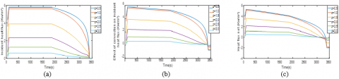
We have presented in Figure 4 (a) the incident heat flux from the waste heat flux resulting from the combustion of palm nut shells. On this profile, we can observe that it has three phases namely: the development of the flame, the equilibrium of the flame and the decay of the flame. The area of the absorber-emitter unit receiving the maximum flux is between 0.5 and 1.5 m for values between 10 and 17 kw.m-2. For Figure 4 (b) and Figure 4 (c), we present the flows taking into account the losses by convection and that due to the radiation of the air. We can also observe the three corresponding phases of the flame. Negative fluxes are obtained, this is due to the fact that after a certain moment the absorber - emitter unit rejects rather than receives it. It is observed that the zone having the most negative value is located on the zone which initially received the maximum heat flow.
Case 2: radiative heat fluxes receive by the absorber for a position of 0.8meter.
For Figure 5(a), Figure 5 (b), Figure 5 (c), it is observed that the profiles have the same behaviors as for Figure 4 (a), Figure 4 (b), Figure 4 (c). What we can see here is the value of the maximum flux received, they are located between 6 and 11.5 kw.m-2, and the area of the absorber - emitter receiving this heat flux is always between 0.5 and 1.5 m.
Case 3: radiative heat fluxes receive by the absorber for a position of 1meter.
When the absorber-emitter is located 1 meter from the heat source, Figure 6(a), Figure 6(b), Figure 6(c), the first observation we can make is to observe that the maximum value is almost 6 kw.m-2. This value is reduced by a third of the value obtained in Figure 4(a), Figure 4(b), Figure 4(c). The three phases of the flame are observed.
Figure 4. (a) incident heat flux, (b) receive heat flux with convection, (c) net heat flux
Figure 5. (a) incident heat flux, (b) receive heat flux with convection, (c) net heat flux
Figure 6. (a) incident heat flux, (b) receive heat flux with convection, (c) net heat flux
Table 2. Maximum heat flux net for different position
|
Distance between flame and TPV absorber (m) |
0.6 |
0.8 |
1 |
|
Maximum net heat flux at the TPV absorber (Kw/m²) |
14.8499 |
10.3568 |
5.2923 |
From Table 2 presented above, we can observe that the maximum net heat flux decreases when the distance between the flame and TPV absorber increases. It can also be seen that at the position 0.6 m, we have the highest maximum net heat flux. This is because the TPV absorber is closed to the flame.
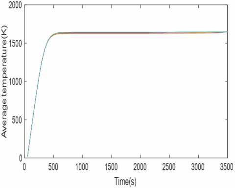
3.2 Evaluation of the average temperature for different position of the absorber to the heat source
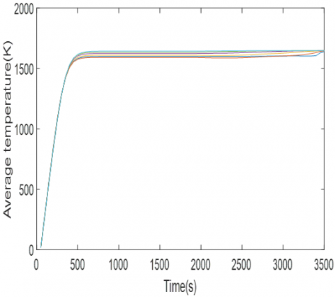
Case 1: average temperature profile at the surface of the absorber for a position of 0.6 meter.
Figure 7. Average temperature profile
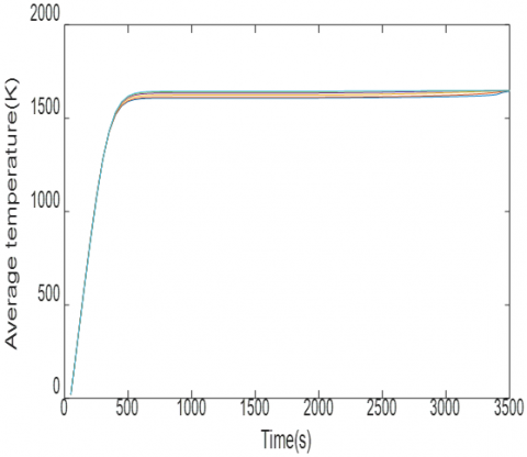
Case 2: average temperature profile at the surface of the absorber for a position of 0.8 meter.
Figure 8. Average temperature profile
Case 3: average temperature profile at the surface of the absorber for a position of 1 meter.
Figure 9. Average temperature profile
In Figure 7, Figure 8, Figure 9 representing respectively the average temperature at the different positions 0.6 m, 0.8 m and 1 m of the absorber, we observe that the maximum value is around 1650k. Between 500s and 3500s for Figure 7, we observe the different temperature profiles for the six positions on the absorber. As for Figure 8 and Figure 9, it can be seen that all the profiles are merged; this shows that the further away from the heat source, the less temperature the absorber receives.
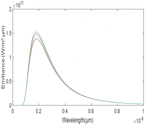
3.3 Evaluation of the emittance for different position of the absorber to the heat source
Case 1: variation of the emittance with the wave length for a position of 0.6 meter of the absorber.
Figure 10. Variation of the emittance with the wave length
Case 2: variation of the emittance with the wavelength for a position of 0.8 meter of the absorber.
Figure 11. Variation of the emittance with the wave length
Case 3: variation of the emittance with the wave length for a position of 1 meter of the absorber.
Figure 12. Variation of the emittance with the wave length
Considering the absorber-emitter as a black body [14, 15], we have represented the emittance as a function of the wavelength. Firstly, the indicator that can be brought out is the value of the wavelength at the extremum of the curve which is around 2000 nm for the three Figure 10, Figure 11, Figure 12. This obtained value is in agreement with the authors [3, 16]. Secondly, we observe that Figure 10 presents the maximum values of the emittance between 12*1010 and 15.5*1010
W.m-2.µm-1 corresponding to the value of λ = 2000 nm; and these values are very distinct. For Figure 11, the values are rather between 13.5*1010 and 15.5*1010 W.m-2.µm-1, and the curves differ very little. In Figure 12 we have a range of values between 14*1010 and 15.5*1010 W.m-2.µm-1 and the curves are very tight. The further away we are from the heat source, the more the value of the emittance increases.
In this work, the waste heat energy resulting from the combustion of palm nut shells has been exploited as a radiative heat source for a TPV absorber system. For that we modeled the flame of combustion using conical approach. Simulations were performed to evaluate the incident and net heat fluxes at the surface of the absorber. The effect of convection and radiative heat lost as well as the position between the absorber and the conical flame, on the heat fluxes profile were analyzed. It comes out that the optimum position where the heat fluxes are maximum is 0.6 m. Moreover, combustion heat lost has an impact on the heat flux. The average temperature was also presented. Regarding the wavelengths, we obtained 2000 nm this value which corresponds to the IR. Finally, results obtained from the numerical simulations shows that radiative waste heat energy from the palm nut shells combustion can be used as radiative heat source for a TPV system.
Thanks to the members of Department of physics, Cameroonian Combustion Group (CCG) for their time, counselling, guidance and availability.
[1] Coutts, T.J. (2001). An overview of thermophotovoltaic generation of electricity. Solar Energy Materials and Solar Cells, 66(1-4): 443-452. https://doi.org/10.1016/S0927-0248(00)00206-3
[2] Rashid, W.E.S.W.A., Ker, P.J., Jamaludin, M.Z.B., Gamel, M.M.A., Lee, H.J., Abd Rahman, N.B. (2020). Recent development of thermophotovoltaic system for waste heat harvesting application and potential implementation in thermal power plant. IEEE Access, 8: 105156-105168. https://doi.org/10.1109/ACCESS.2020.2999061
[3] Mbakop, F.K., Tom, A., Dadjé, A., Vidal, A.K.C., Djongyang, N. (2020). One-dimensional comparison of Tio2/SiO2 and Si/SiO2 photonic crystals filters for thermophotovoltaic applications in visible and infrared. Chinese Journal of Physics, 67: 124-134. https://doi.org/10.1016/j.cjph.2020.06.004
[4] Woolf, D.N., Kadlec, E.A., Bethke, D., Grine, A.D., Nogan, J.J., Cederberg, J.G., Hensley, J.M. (2018). High-efficiency thermophotovoltaic energy conversion enabled by a metamaterial selective emitter. Optica, 5(2): 213-218. https://doi.org/10.1364/OPTICA.5.000213
[5] Piness-Sommer, M., Braun, A., Katz, E.A., Gordon, J.M. (2016). Ultra-compact combustion-driven high-efficiency thermophotovoltaic generators. Solar Energy Materials and Solar Cells, 157: 953-959. https://doi.org/10.1016/j.solmat.2016.08.018
[6] Ferrari, C., Melino, F., Pinelli, M., Spina, P.R., Venturini, M. (2014). Overview and status of thermophotovoltaic systems. Energy Procedia, 45: 160-169. https://doi.org/10.1016/j.egypro.2014.01.018
[7] Bendelala, F., Cheknane, A., Hilal, H. (2018). Enhanced low-gap thermophotovoltaic cell efficiency for a wide temperature range based on a selective meta-material emitter. Solar Energy, 174: 1053-1057. https://doi.org/10.1016/j.solener.2018.10.006
[8] Mbakop, F.K., Djongyang, N., Ejuh, G.W., Raїdandi, D., Woafo, P. (2017). Transmission of light through an optical filter of a one-dimensional photonic crystal: application to the solar thermophotovoltaic system. Physica B: Condensed Matter, 516: 92-99. https://doi.org/10.1016/j.physb.2017.04.033
[9] Licht, A.S., Shemelya, C.S., DeMeo, D.F., Carlson, E.S., Vandervelde, T.E. (2017). Optimization of GaSb thermophotovoltaic diodes with metallic photonic crystal front-surface filters. 2017 IEEE 60th International Midwest Symposium on Circuits and Systems (MWSCAS), Boston, MA, USA, pp. 843-846. https://doi.org/10.1109/MWSCAS.2017.8053055
[10] Sakakibara, R., Stelmakh, V., Chan, W.R., Ghebrebrhan, M., Joannopoulos, J.D., Soljacic, M., Čelanović, I. (2019). Practical emitters for thermophotovoltaics: A review. Journal of Photonics for Energy, 9(3): 032713. https://doi.org/10.1117/1.JPE.9.032713
[11] Chubb, D. (2007). Fundamentals of Thermophotovoltaic Energy Conversion. Elsevier.
[12] Franssen, J.M., Zaharia, R. (2005). Design of Steel Structures subjected to Fire. Background and Design Guide to Eurocode 3. Les Editions de l'Universite de Liege.
[13] Howell, J.R., Siegel, R., Pinar Mengüç, M. (2011). Thermal Radiation Heat Transfer-Fifth Edition, CRC Press, 151-204.
[14] Cristina, P.A. (2012). The Optical Transmission of One-Dimensional Photonic Crystals Containing Double-Negative Materials. Photonic Crystals: Innovative Systems, Lasers and Waveguides, 41.
[15] Liu, G., Xuan, Y., Han, Y., Li, Q. (2008). Investigation of one-dimensional Si/SiO2 hotonic crystals for thermophotovoltaic filter. Science in China Series E: Technological Sciences, 51(11): 2031-2039. https://doi.org/10.1007/s11431-008-0139-0
[16] Mbakop, F.K., Djongyang, N., Raїdandi, D. (2016). One–dimensional TiO 2/SiO2 photonic crystal filter for thermophotovoltaic applications. Journal of the European Optical Society-Rapid Publications, 12(1): 23. https://doi.org/10.1186/s41476-016-0026-4