Meng Zhang* | Xutong Wang
© 2021 IIETA. This article is published by IIETA and is licensed under the CC BY 4.0 license (http://creativecommons.org/licenses/by/4.0/).
OPEN ACCESS
Improving the energy use efficiency of the energy system is of great significance to the development of the national energy economy and the improvement of the national economic competitiveness. The existing domestic research on thermo-economic costs is insufficient. For example, there is no research on the allocation of thermo-economic costs and on the complex energy network with multiple energy outputs. Therefore, this paper reconstructs and optimizes the thermo-economic cost analysis model for the complex energy network. First, the thermo-economic cost model for each sub-network and that for each energy output of the complex energy network were established, and the structure block diagram of the distributed thermo-economic cost allocation model for the complex energy network was given. Then, a local-global decomposition optimization method was proposed for the complex energy network to achieve the thermo-economic optimization of the complex energy network. The experimental results proved the effectiveness of the proposed algorithm.
complex energy network, thermo-economic cost analysis, model optimization, exergy cost analysis
The energy industry is the material basis for modernization, and establishing an energy supply network with high security and high reliability should be a core development strategy, whether in a developed or developing country [1-4]. Improving the energy use efficiency of the energy system is of great significance to the development of the national energy economy and the improvement of the national economic competitiveness [5-9]. Currently, the analysis of the energy network with various forms of heat-work conversion is mainly based on the theory of thermodynamic analysis. In the energy conservation analysis and optimization of the complex energy network, the traditional analysis technology cannot quantify the irreversible loss in the energy production process, while the thermo-economic analysis method, which introduces the concept of cost, can solve the above problem [10-16].
Ghorbani et al. [17] developed and analyzed an integrated energy system consisting of photovoltaic collectors, a jet refrigeration cycle and phase-change material storage. The power and refrigeration capacities of the proposed system are about 6666 kW and 5395 kW, respectively. Through energy and exergy analysis, it was found that the total heat efficiency and the total exergy efficiency of the system were approximately 60.51% and 50.84%, respectively. Yue et al. [18] compared the overall thermal and economic performance of the vehicle energy supply system with an independent organic Rankine cycle subsystem for waste heat recovery and the traditional vehicle energy supply system, and verified that the proposed system has significant advantages in both thermal and economic performance. Owebor et al. [19] proposed an energy, exergy, environmental and economic analysis model for municipal waste-to-energy plants, and generate the solution and simulation of the model in Gasify, Engineering Equation Solver and MS Excel. Ogorure et al. [20] introduced an energy, exergy, environmental and economic analysis method for multi-generation plants that use agricultural waste to generate power, and put forward the energo environmental sustainability and economic sustainability indexes to comprehensively evaluate the sustainability of the proposed power plant. Favre et al. [21] proposed a method that can optimize the coupling relationship between the local renewable energy production system and the energy storage equipment and different users like buildings and their peripheral equipment. The optimization criteria include the independence of renewable energy and the ecological and economic costs. Zhu et al. [22] proposed three integration schemes for the hybrid energy system, performed thermo-economic analysis of the three schemes with the trough solar and thermal power units as examples, and calculated the LEC of the solar optimization scheme.
Currently, the research on thermo-economic costs at home and abroad focuses on the specific application of 4 models like the accounting model, the matrix model, the structural model and the optimization model, while little has been done on the allocation of thermo-economic costs and the complex energy network with multiple energy outputs. Therefore, a thermo-economic cost analysis model was reconstructed and optimized for the complex energy network in this paper. The main content of this paper is as follows: 1) A thermo-economic cost model was constructed for each sub-network of the complex energy network; 2) a thermo-economic cost model was constructed for each energy output of the complex energy network; 3) the structural block diagram of the distributed thermo-economic cost allocation model for the complex energy network was given; 4) a local-global decomposition optimization method was proposed for the complex energy network to complete the thermo-economic optimization of the complex energy network; 5) the process flow of the thermo-economic optimization algorithm was provided for the complex energy network; 6) An experiment was conducted to verify the effectiveness of the proposed algorithm.
Let the unit thermo-economic cost of the exergy flow in the complex energy network be denoted as ξ, the event matrix describing the relationship between the energy sub-network and each exergy flow be denoted as D, and the exergy cost of the complex energy network as E. For a given complex energy network, the distribution of the exergy flows in the network and the structure of the sub-networks are known. Based on the reasoning process of the exergy cost calculation matrix, first n exergy cost balance equations are listed for n sub-networks, and according to the idea of block matrix, the following equation is formed:
$D\times \xi +E=0$ (1)
Since the number of sub-networks n is always smaller than the number of exergy flows m, if the calculation matrix is required to have one unique solution, it is necessary to establish (m-n) supplementary equations to make it full rank. Assuming that the supplementary event matrix is represented by β, that the unit exergy cost by eσ, and that the column vector by σ, the supplementary equation is shown in Eq. (2):
$\beta \times \xi -\left[ {{e}_{\sigma }}\sigma \right]=0$ (2)
The formed calculation matrix of (m, m) is shown in Eq. (3):
${{D}^{*}}\times \xi +{{E}^{*}}=0$ (3)
where,
${{E}^{*}}=\left[ \begin{align} & E \\ & -{{e}_{\sigma }}\sigma \\\end{align} \right]$ (4)
Assuming that D is an invertible matrix, the unit thermo-economic cost ξ of exergy flow in the complex energy network can be obtained as follows:
$\xi =-{{D}^{*}}^{-1}\times {{E}^{*}}$ (5)
The calculation formula of the total thermo-economic cost of exergy flows in the complex energy network is expressed in Eq. (6):
${{\xi }^{*}}=-{{\left( {{C}_{G}} \right)}^{*}}^{-1}\times {{D}^{*}}^{-1}\times {{E}^{*}}$ (6)
Different forms of energy have different exergy values and are subject to different influencing factors (Table 1). For example, the exergy values of fossil fuels are mainly calculated based on environmental parameters and their components, while the exergy value of solar energy is determined by the solar radiation area, and that of wind energy by the wind force, and that of biomass energy depends on the specific biological material. It is not appropriate to input all forms of energy into the complex energy network based on the concept of exergy only.
Regarding the allocation of thermo-economic costs between sub-networks or exergy flows, it is important to consider the inequivalence of exergy and divide the costs into two parts: the allocation of energy costs and non-energy costs. Assuming that the i-th sub-network has a total of j exergy flows, with a unit exergy price of ei,j, the specific exergy cost of this sub-network can be defined as the internal average unit price of all input exergy flows in the sub-network, calculated according to Eq. (7):
${{\hat{C}}_{i}}=\frac{\sum{{{C}_{i,j}}{{e}_{i,j}}}}{\sum{{{C}_{i,j}}}}$ (7)
The non-energy cost allocated to the unit exergy cost of the input exergy flows in the i-th sub-network is defined as the specific non-energy cost of the sub-network, calculated according to Eq. (8):
${{\hat{E}}_{mi}}=\frac{\sum{{{E}_{mi}}}}{\sum{{{C}_{i,j}}}}$ (8)
Assuming that the exergy efficiency of the j-th exergy flow in the i-th sub-network is represented by δi,j, the corresponding calculation formula of unit exergy cost is expressed as Eq. (9):
${{\hat{e}}_{i,j}}=\frac{{{{\hat{C}}}_{i}}+{{{\hat{E}}}_{ni}}}{{{\delta }_{i,j}}}$ (9)
Assuming that the growth factor of the unit exergy cost of the j-th exergy flow in the i-th sub-network is represented by αi,j, the unit exergy cost also satisfies:
${{\hat{e}}_{i,j}}={{\alpha }_{i,j}}{{e}_{im}}$ (10)
αi,j can be expressed as:
${{\alpha }_{i,j}}=\frac{{{{\hat{e}}}_{i,j}}}{{{e}_{im}}}=\frac{{{{\hat{C}}}_{i}}+{{{\hat{E}}}_{mi}}}{{{\delta }_{i,j}}}$ (11)
From the above formula, αi,j is determined by the specific energy cost ei*, the specific non-energy cost Emi*, the exergy efficiency δi,j and the unit price of input exergy ei,j. In particular, αi,j is directly proportional to the total exergy cost of the network, and inversely proportional to δi,j.
Table 1. Unit exergy costs of different forms of energy
|
Energy |
Coal |
Natural gas |
Solar energy |
Wind energy |
Biomass energy |
Electric energy |
|
Exergy value |
26756 |
51998 |
363 |
3400 |
17534 |
3500 |
|
Price |
475 |
4132.8 |
/ |
/ |
320 |
618.25 |
|
Unit exergy cost |
18.23 |
82.31 |
/ |
/ |
19.72 |
172.31 |
Figure 1. Thermo-economic cost allocation model for a single-input multi-output energy network
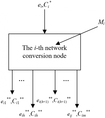
If the energy network under study is a traditional network with a single energy input and multiple energy outputs, the proportion of output energy can be ignored in the thermo-economic cost allocation analysis, and only the total amount of output exergy is considered. Figure 1 shows the thermo-economic cost allocation model for the network. Assuming that the input exergy flow into the i-th network conversion node of the network during the study period is represented by Ci*, that the unit price of the output exergy flow at this node by Te, and that the j-th output exergy flow of this node by Cij**, the constructed exergy transformation model can be expressed as Eq. (12):
${{T}_{e}}=\frac{e_{i}^{*}C_{i}^{*}+{{M}_{i}}}{\sum\limits_{j=1}^{m}{C_{ij}^{**}}}$ (12)
Based on the traditional exergy cost allocation method, the cost of the output exergy at a node of this type of energy network can be regarded as approximately equal, then:
${{T}_{e1}}={{T}_{e2}}=...={{T}_{ei}}=...{{T}_{el}}={{T}_{e}}$ (13)
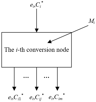
In this type of energy network, whether exergy is output in the form of electricity, heat, gas or cold, the output exergy can still be divided into primary and auxiliary ones. Although the cost of output exergy is equal, the cost of the main input exergy can be easily underestimated and the necessity of auxiliary output energy overestimated. Therefore, this paper established a distributed thermo-economic cost allocation model for the complex energy network that fully considers the proportion of primary and auxiliary energy output, and set the following two rules for this type of cost allocation problem:
1) The energy cost of the network input exergy is all allocated to the cost of the primary output exergy and no cost is allocated to the auxiliary output energy;
2) The non-energy costs are allocated to the main and auxiliary output exergy according to the different types of equipment and labor, etc.
Figure 2. Distributed thermo-economic cost allocation model for the complex energy network
Figure 2 shows the distributed thermo-economic cost allocation model for the complex energy network. Suppose that the primary output exergy of the distributed complex energy network exergy conversion model is the 1-h-th output exergy, and that the auxiliary output exergy is the remaining h+1-m-th output exergy. Let the exergy flow entering the i-th network conversion node during the study period be denoted as Ci*, the total flow of the primary and auxiliary output exergy at the corresponding node as Σmp=1Cik**, the total flow of the primary output exergy as Σhl=1Cil**, and the non-energy cost of the output exergy at this node as Mi, and then the thermo-economic cost calculation formula for the primary output exergy is expressed as Eq. (14):
${{T}_{e}}=\frac{e_{i}^{*}C_{i}^{*}}{\sum\limits_{l=1}^{h}{C_{il}^{**}}}+\frac{{{M}_{i}}}{\sum\limits_{k=1}^{m}{C_{ip}^{**}}},i=1,2,...,h$ (14)
Assuming that the j-th auxiliary output exergy flow at the i-th network conversion node during the study period is represented by Cij**, and that the non-energy cost of the output exergy flow at this node by Mi, the thermo-economic cost calculation formula for theauxiliary output exergy is expressed as Eq. (15):
${{T}_{e}}=\frac{{{M}_{i}}}{\sum\limits_{p=1}^{m}{C_{ip}^{**}}},i=\left( h+1 \right),...,m\text{ }$ (15)
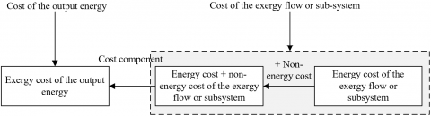
In summary, the distributed thermo-economic cost allocation model for the complex energy network proposed in this paper consists of the energy cost model for each exergy flow or sub-network, the energy cost + non-energy cost model for each exergy flow or sub-network and the exergy cost model for each form of output energy. The exergy cost model for each form of output energy based on the first two layers of models can be used to calculate the exergy cost of each energy output and provide a reference for its pricing (Figure 3).
Figure 3. Distributed thermo-economic cost allocation model for the complex energy network
The thermo-economic analysis method, which has introduced the concept of cost, can help expand the thermo-economic cost allocation problem of the complex energy network. However, with the continuous development of the energy industry, the internal structure of the energy network has become more complex and contained more parameters. When the global optimization method is used to solve the problem, the convergence speed will be very slow due to the restriction of the constraint equation. If the complex energy network is decomposed into several sub-networks and locally optimized, the convergence speed will be faster, but usually the true global optimum cannot be achieved.
In view of the problems of global optimization and local optimization, this paper constructed a local-global decomposition optimization method suitable for the complex energy network. In this method, all sub-networks are divided based on the degree of coupling between the sub-networks, and those with a higher degree of coupling are divided into one group; each group is locally optimized, and the sub-networks with a lower degree of coupling are combined and then globally optimized. Based on this method, the complex energy network can approach the thermo-economic optimality conditions as fast as possible.
4.1 Construction of the optimization model
The constructed thermo-economic cost allocation optimization model for the complex energy network aims to optimize the overall cost allocation objective under certain restrictions or constraints. The model consists of two parts: constraint conditions and the optimization objective. The mathematical expression of the model optimization objective is shown in Eq. (16):
$\underset{a}{\mathop{min}}\,g\left( a \right)$ (16)
where, the independent variable set of the complex energy network is denoted as a:
$a=\left( {{a}_{1}},{{a}_{2}},...,{{a}_{m}} \right)$ (17)
a is subject to the equality constraint fi due to the mass balance, energy balance, and physical and chemical mechanism equations of the process:
${{f}_{i}}\left( a \right)=0\text{ }i=1,2,...,n$ (18)
At the same time, it is subject to the inequality constraint hi due to the limits, security, stability, and environmental requirements of the network design and operation:
${{h}_{j}}\left( a \right)\le 0\text{ }j=1,2,...,v$ (19)
a can be divided into three subsets, namely the independent variable subset p used for operation optimization, the independent variable subset q for design optimization, and the independent variable subset r for comprehensive optimization:
$a=\left( p,q,r \right)$ (20)
where, p represents such independent variables as load factor, mass flow, pressure and temperature, q represents such independent variables as unit load, isentropic efficiency, heat difference of heater, and r represents whether the sub-network has an optimal process structure or binary-state variable in the configuration. Each sub-network has a corresponding r. The objective function shown in Eq. (16) can be transformed into:
$\underset{p,q,r}{\mathop{min}}\,g\left( p,q,r \right)$ (21)
For a given complex energy network, r is known at this time, and the cost allocation optimization of the network only involves design optimization and operation optimization:
$\underset{p,q}{\mathop{min}}\,{{g}_{S}}\left( p,q \right)$ (22)
If the network structure and operation requirements are known, that is, r and q are known, the cost allocation optimization of the network only involves operation optimization:
$\underset{p}{\mathop{min}}\,{{g}_{UH}}\left( p \right)$ (23)
In order to reduce the complexity of the thermo-economic cost allocation optimization of the complex energy network, the optimum synthesis of the network is ignored. It is determined that all equipment except generators and condensers are within the optimization range of the complex energy network, including boilers, steam turbines, heat exchangers and water pumps, etc. Let the thermodynamic efficiency of a boiler be denoted as ΦGL, that of a steam turbine as ΦMO, that of a heat exchanger and a water pump as ΦHE and ΦWP, the heat difference at the feed outlet of a heater as WSEHO, and the temperature of the boiler main steam and the reheat steam as ψZQ. The characteristic variables related to the design and operation of equipment, such as efficiency, heat difference, and temperature, can be taken as the independent variable a of the network:
$\begin{align} & a=\left( {{\Phi }_{GL}} \right.,{{\Phi }_{MO11}},{{\Phi }_{MO12}},{{\Phi }_{MO13}},{{\Phi }_{MO14}},{{\Phi }_{MO21}}, \\ & {{\Phi }_{MO22}},{{\Phi }_{MO23}},{{\Phi }_{MO31}},{{\Phi }_{MO32}},{{\Phi }_{HE}},{{\Phi }_{WP}},WS{{E}_{HO1}}, \\ & WS{{E}_{HO2}},WS{{E}_{HO3}},WS{{E}_{HO4}},WS{{E}_{HO5}},WS{{E}_{HO6}},\left. {{\psi }_{ZQ}} \right) \\\end{align}$ (24)
4.2 Global optimization
Under the condition that the economic environmental factors such as the interest rate and the inflation rate and the physical environmental factors such as the annual operating hours of the complex energy network are fixed, the global optimization of the complex energy network can be expressed as the minimization of the external resources ER consumed by the network and the total investment IN, that is, the minimization of the total annual cost of the network Ψ, through the adjustment of the internal independent variable a of the network under a certain net load. Assuming that the unit price of the external fuel is represented by oER,i and that the amortization factor by μ, then:
$\underset{a}{\mathop{min}}\,\Psi ={{\Psi }_{RL}}+{{\Psi }_{IN}}=\sum\limits_{i=1}^{c}{{{o}_{ER,i}}E{{R}_{i}}}+\mu \sum\limits_{s=1}^{n}{I{{N}_{s}}}$ (25)
Assuming that the dependent variables including the temperature, pressure, flow rate, and specific enthalpy of each exergy flow are represented by b=(b1, b2, …, bl), and that the constraint equation that characterizes the features of quality, energy, and equipment of the complex energy network by fj(a,b), the independent variable a is subject to the equality constraint fi(a, b):
${{f}_{j}}\left( a,b \right)=0,\text{ }j=1,...,J$ (26)
Assuming that the constraint equation that characterizes the security, stability and environmental requirements of the complex energy network is represented by hl(a, b), a is subject to the inequality constraint hl:
${{h}_{l}}\left( a,b \right)\le 0,\text{ }l=1,...,L$ (27)
The external fuel consumption in the objective function can be determined by the function shown in Eq. (28):
$E{{R}_{i}}=E{{R}_{i}}\left( a,b \right),\text{ }i=1,...,t$ (28)
The investment cost in the objective function can be determined by the function shown in Eq. (29):
$I{{N}_{s}}=I{{N}_{s}}\left( a,b \right),\text{ }s=1,...,n$ (29)
The external fuel consumption function ERi(a, b) of the complex energy network under study is determined by the fuel-output model. The equipment investment cost estimation equation INψ(a, b) for the complex energy network characterizes the correlation between the investment cost IN and the network variables (a, b).
Once the optimization model for the complex energy network consisting of the objective function and the inequality constraint is determined, the nonlinear optimization algorithm can be used in the optimization processing of the optimization model to find the optimal solution a* of the independent variable a of the complex energy network and the value of the corresponding dependent variable b.
4.3 Local optimization
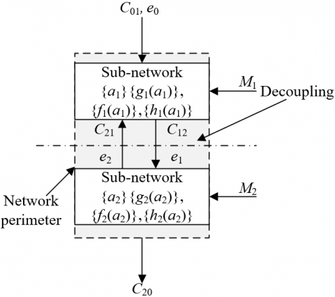
If the output exergy of a sub-network and the unit cost of the resources consumed by the sub-network are known and do not change with the independent variables of the sub-network, then it can be determined that this sub-network is in a thermo-economic isolation condition. Through the decomposition of the sub-networks, each sub-network and piece of equipment will meet this condition, that is, there is no need to consider multiple equipment or sub-networks, but only a single sub-network or piece of equipment needs to be optimized, and the solution obtained thereby can also ensure the global optimization (Figure 4).
Figure 4. Schematic diagram of network decoupling during local optimization
Let the set of local variables that only affect the j-th sub-network be denoted as a, and the set of dependent variables as b. Let the unit thermo-economic cost of the j-th sub-network output be denoted as ej, the sub-network technical output coefficient involving the unit exergy and the exergy flow rate as lij, and the thermo-economic cost of the unit output exergy as lINj=μINj/Cj. When the independent variable a only affects a single sub-network, the objective function for minimizing the thermo-economic cost of the output is expressed as Eq. (30):
$\underset{a}{\mathop{min}}\,\Psi ={{e}_{j}}{{C}_{j}}=\left( \sum\limits_{i=0}^{n}{{{l}_{ij}}\left( a,b \right)}{{e}_{j}}+lI{{N}_{j}}\left( a,b \right) \right){{C}_{j}}$ (30)
When multiple sub-networks and even the global complex energy network are affected by the independent variable a, the objective function for minimizing the sum of the thermo-economic costs of the output exergy from all affected sub-networks is expressed as Eq. (31):
$\underset{a}{\mathop{min}}\,\Psi =\sum\limits_{j=1}^{n}{{{e}_{j}}{{C}_{j}}}=\sum\limits_{j=1}^{n}{\left( \sum\limits_{j=1}^{n}{{{l}_{ij}}\left( a,b \right)}{{e}_{j}}+lI{{N}_{j}}\left( a,b \right) \right){{C}_{j}}}$ (31)
Let ej and Cj in the optimization process of Eq. (30) and Eq. (31) be constants. From the above analysis, it can be seen that, before constructing the thermo-economic cost allocation optimization objective function for the complex energy network, it is important to first determine the properties of the independent variables of the complex energy network and then determine the objective function based on the analysis results of the properties. Based on the thermo-economic cost equation, this paper explored the disturbing influence of the independent variable a on the thermo-economic cost of each sub-network, and obtained:
$\Delta e_{0,j}^{a}=\left( \sum\limits_{i=0}^{m}{{{e}_{j}}}\frac{\partial {{l}_{ij}}}{\partial a}+\frac{\partial l\cdot I{{N}_{j}}}{\partial a} \right){{C}_{j}}\Delta a$ (32)
The proportion τja of the variation to the thermo-economic cost of the j-th sub-network caused by the independent variable a in the total cost variation can be expressed by Eq. (33):
$\tau _{j}^{a}=\frac{\left| \Delta e_{0,j}^{a} \right|}{\sum\limits_{i=1}^{m}{\left| \Delta e_{0,j}^{a} \right|}}\times 100$ (33)
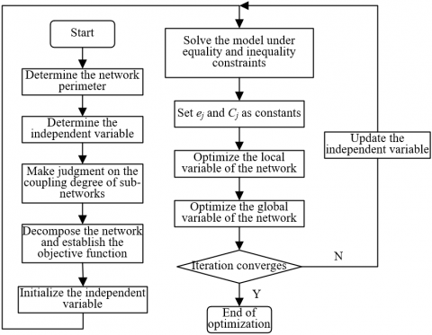
When τja approaches 1, the independent variable a is a local variable of the j-th sub-network, and when τja is between 0 and 1, the independent variable a is a global variable. Based on τja, the degree of coupling between sub-networks can be quantified. Figure 5 shows the process flow of the thermo-economic optimization algorithm for the complex energy network.
This paper added the calculated unit exergy cost of each sub-network with its unit non-energy cost to obtain the unit thermo-economic cost of each sub-network. The energy outputs of the complex energy network were grouped indiscriminately into 6 groups: G1, G2, G3, G4, G5 and G6. The calculation results obtained by Method 1 (the traditional calculation method), Method 2 (which introduces the energy quality coefficient) and Method 3 (which introduces the exergy reduction coefficient) are given in Table 2, Table 3, and Table 4, respectively.
Figure 5. Process flow of the thermo-economic optimization algorithm for the complex energy network
Table 2. Unit thermo-economic cost of each sub-network under Method 1
|
Sub-network group |
G1 |
G2 |
G3 |
G4 |
G5 |
G6 |
|
Unit exergy cost |
38.65 |
21.76 |
0 |
0 |
47.96 |
103.61 |
|
Unit non-energy cost |
4.53 |
3.62 |
101.59 |
52.62 |
10.74 |
4.23 |
|
Unit thermo-economic cost |
41.42 |
53.44 |
101.59 |
53.78 |
24.31 |
105.39 |
Table 3. Unit thermo-economic cost of each sub-network under Method 2
|
Sub-network group |
G1 |
G2 |
G3 |
G4 |
G5 |
G6 |
|
Unit exergy cost |
86.25 |
47.36 |
0 |
0 |
108.92 |
175.47 |
|
Unit non-energy cost |
4.35 |
3.72 |
102.68 |
85.91 |
11.75 |
4.25 |
|
Unit thermo-economic cost |
92.38 |
54.64 |
102.68 |
85.91 |
118.57 |
187.32 |
Table 4. Unit thermo-economic cost of each sub-network under Method 3
|
Sub-network group |
G1 |
G2 |
G3 |
G4 |
G5 |
G6 |
|
Unit exergy cost |
88.53 |
16.78 |
0 |
0 |
22.36 |
95.79 |
|
Unit non-energy cost |
4.35 |
3.62 |
100.38 |
82.61 |
1072 |
4.19 |
|
Unit thermo-economic cost |
92.36 |
17.25 |
100.38 |
82.61 |
32.41 |
101.53 |
Based on the obtained unit thermo-economic cost of each sub-network, the thermo-economic cost of each energy output considering the proportions of primary and auxiliary energy outputs was further calculated.
In this paper, the energy outputs of the complex energy network studied were classified into six categories, namely coal (C), natural gas (GNG), solar energy (SE), wind energy (WE), biomass energy (BE), and electric energy (E). Table 1 shows the unit exergy costs of different forms of energy. The thermo-economic costs of different energy outputs are different. Below is how the unit thermo-economic cost of each category of energy output was determined according to the way each category of energy is generated. The thermo-economic cost allocation method considering the proportions of primary and auxiliary energy outputs proposed in this paper was adopted for cost allocation.
Since only the energy output of the primary energy conversion process is considered, the unit thermo-economic cost of the equipment used in the energy conversion process is the unit thermo-economic cost of the energy, without any need for allocation. For energy output beyond primary energy conversion, all unit exergy costs should be allocated to the primary energy source. Based on the above operations, the unit exergy cost, unit non-energy cost, and unit thermo-economics cost of each sub-network were allocated to the 6 categories of energy outputs. Table 5 shows the thermo-economic cost of each sub-network obtained by the proposed allocation method 4.
After the introduction of the energy quality coefficient, the thermo-economic cost of each sub-network was also allocated to the 6 categories of energy outputs. Table 6 shows the calculation result of the thermo-economic cost of each sub-network obtained by the proposed allocation method 5 after the introduction of the energy quality coefficient. Similarly, Table 7 shows the calculation result of the thermo-economic cost of each sub-network obtained by the proposed allocation method 5 after the introduction of the exergy reduction coefficient.
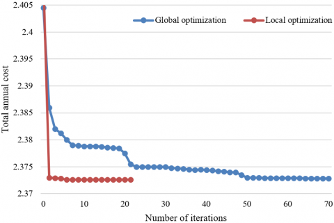
The iterations in global optimization and local optimization of the thermo-economics of the complex energy network studied started with the same initial value. Figure 6 shows the iterative convergence of global optimization and local optimization. It can be seen that the local-global decomposition optimization method proposed in this paper for the complex energy network had a higher convergence rate. After 2 to 3 iterations, the total thermo-economic cost basically stabilized. The optimization algorithm proposed in this paper took about half of the time consumed by the traditional global optimization algorithm.
Table 5. Thermo-economic cost of each sub-network under Method 4
|
Sub-network |
C |
GNG |
SE |
WE |
BE |
E |
|
Unit exergy cost |
89.23 |
16.84 |
0 |
0 |
22.35 |
82.91 |
|
Unit non-energy cost |
4.35 |
3.62 |
101.84 |
85.21 |
10.75 |
4.26 |
|
Unit thermo-economic cost |
95.37 |
19.25 |
101.84 |
85.21 |
32.61 |
86.75 |
Table 6. Thermo-economic cost of each sub-network under Method 5
|
Sub-network |
C |
GNG |
SE |
WE |
BE |
E |
|
Unit exergy cost |
85.26 |
47.36 |
0 |
0 |
108.22 |
135.31 |
|
Unit non-energy cost |
4.65 |
3.62 |
102.36 |
85.41 |
10.75 |
4.25 |
|
Unit thermo-economic cost |
91.64 |
53.84 |
102.36 |
85.41 |
112.57 |
136.72 |
Table 7. Thermo-economic cost of each sub-network under Method 6
|
Sub-network |
C |
GNG |
SE |
WE |
BE |
E |
|
Unit exergy cost |
86.53 |
16.84 |
0 |
0 |
22.56 |
82.31 |
|
Unit non-energy cost |
4.53 |
3.62 |
102.58 |
85.21 |
10.75 |
4.26 |
|
Unit thermo-economic cost |
92.56 |
17.23 |
102.58 |
85.21 |
32.41 |
86.75 |
Table 8. Thermodynamic and exergy analysis results under optimal conditions
|
No. |
1 |
2 |
3 |
4 |
5 |
6 |
7 |
|
Mass flow rate |
868.75 |
57.23 |
812.35 |
67.32 |
722.35 |
722.35 |
32.76 |
|
Pressure |
17.32 |
5.777 |
3.642 |
3.642 |
3.642 |
3.267 |
1.753 |
|
Specific enthalphy |
3484.23 |
3169.48 |
3028.65 |
3053.21 |
3053.21 |
3679.28 |
3541.94 |
|
Specific exergy |
1562.75 |
1372.85 |
1123.54 |
1123.54 |
1156.32 |
1579.63 |
1108.86 |
|
No. |
8 |
9 |
10 |
11 |
12 |
13 |
14 |
|
Mass flow rate |
61.84 |
27.63 |
32.55 |
32.55 |
678.26 |
37.28 |
26.31 |
|
Pressure |
0.835 |
0.835 |
0.835 |
0.006 |
0.835 |
0.362 |
0.128 |
|
Specific enthalphy |
3127.65 |
3127.65 |
3127.65 |
2568.52 |
3244.26 |
2871.9 |
2754.68 |
|
Specific exergy |
1002.32 |
1002.32 |
1002.32 |
153.21 |
1025.69 |
796.35 |
582.08 |
|
No. |
15 |
16 |
17 |
18 |
19 |
20 |
21 |
|
Mass flow rate |
28.92 |
31.54 |
569.3 |
682.49 |
685.24 |
685.24 |
685.24 |
|
Pressure |
0.065 |
0.063 |
0.027 |
0.006 |
1.725 |
1.725 |
1.725 |
|
Specific enthalphy |
2852.31 |
2695.74 |
2231.56 |
185.92 |
146.21 |
268.2 |
369.51 |
|
Specific exergy |
484.23 |
798.66 |
581.45 |
1.6 |
3.08 |
15.21 |
27.63 |
|
No. |
22 |
23 |
24 |
25 |
26 |
27 |
28 |
|
Mass flow rate |
685.24 |
685.24 |
885.61 |
885.61 |
885.61 |
885.61 |
885.61 |
|
Pressure |
1.725 |
1.725 |
0.9 |
18.753 |
18.753 |
18.753 |
18.753 |
|
Specific enthalphy |
453.21 |
565.23 |
729.54 |
719.53 |
889.64 |
1032.75 |
1231.82 |
|
Specific exergy |
47.51 |
78.29 |
125.9 |
143.85 |
185.76 |
265.32 |
319.25 |
|
No. |
29 |
30 |
31 |
32 |
33 |
34 |
35 |
|
Mass flow rate |
56.23 |
125.76 |
159.25 |
34.21 |
59.76 |
85.1 |
115.72 |
|
Pressure |
5.796 |
3.544 |
1.508 |
0.367 |
0.125 |
0.062 |
0.021 |
|
Specific enthalphy |
1086.75 |
892.65 |
765.28 |
475.35 |
371.56 |
284.21 |
165.29 |
|
Specific exergy |
302.43 |
316.94 |
137.8 |
51.26 |
32.06 |
16.8 |
2.65 |
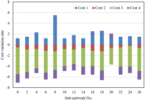
The thermodynamic and exergy analysis results of the complex energy network under the optimal conditions are given in Table 8. Figure 7 shows the unit thermo-economic costs of each of the 26 ungrouped sub-networks under the optimal operating conditions, including Cost 1 (investment cost), Cost 2 (specific negentropy cost), Cost 3 (specific irreversible cost), and Cost 4 (energy cost). Through comparison with the results of the previous thermo-economic cost analysis, it can be found that local optimization of thermo-economics reduced the total investment cost of the complex energy network by about 4%, and that the exergy cost and thermo-economic cost of the energy output from each sub-network also saw certain changes.
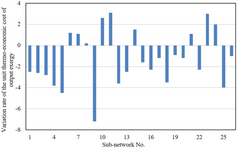
This paper analyzed the variations in and influencing factors to the unit thermo-economic cost of the energy output from each sub-network before and after the thermo-economic optimization of the complex energy network. Figure 8 shows the variations in the unit thermo-economic cost of the energy output from each sub-network before and after the thermo-economic optimization, and Figure 9 shows the analysis results of the factors influencing the variations in the thermo-economic cost of each sub-network before and after the thermo-economic optimization. It can be seen that the unit thermo-economic cost of the energy output from most of the sub-networks was reduced by 1-2%, and that among the 26 ungrouped sub-networks, Sub-network 8 had the largest decrease, reaching 7.1%. The main influencing factor that caused the thermo-economic cost reduction of these sub-networks is the improvement of the thermal performance of the equipment, which reduced the irreversible cost of the four costs. The cost reduction of boilers, steam turbines and other equipment mainly led to the significant reduction of the energy cost among the four costs.
Figure 6. Iterative convergence of global optimization and local optimization
Figure 7. Unit thermo-economic cost of each sub-network under the optimal conditions
Figure 8. Variations in the unit thermo-economic cost of the energy output from each sub-network before and after the thermo-economic optimization
Figure 9. Influencing factors to the variations in the thermo-economic cost of each sub-network before and after the thermo-economic optimization
This paper reconstructed and optimized the thermo-economic cost analysis model for the complex energy network. First, the thermo-economic cost model for each sub-network of the complex energy network and that for each energy output were constructed, and then, a block diagram of the distributed thermo-economic cost allocation model for the complex energy network was given. Next, a local-global decomposition optimization method suitable for the complex energy network was proposed to complete the thermo-economic optimization of the complex energy network. The experiment showed the calculation results of the unit exergy cost, unit non-energy cost and unit thermo-economic cost obtained by the traditional calculation method and the proposed local-global decomposition optimization method. The iterative convergence curves of global optimization and local optimization were drawn, and the variations in and influencing factors to the unit thermo-economic cost of the energy output from each sub-network of the complex energy network before and after thermo-economic optimization were analyzed, which proved the effectiveness of the proposed algorithm.
[1] Ahn, J., Cho, S., Chung, D.H. (2017). Analysis of energy and control efficiencies of fuzzy logic and artificial neural network technologies in the heating energy supply system responding to the changes of user demands. Applied Energy, 190: 222-231. https://doi.org/10.1016/j.apenergy.2016.12.155
[2] Shafiei Kaleibari, S., Gharizadeh Beiragh, R., Alizadeh, R., Solimanpur, M. (2016). A framework for performance evaluation of energy supply chain by a compatible network data envelopment analysis model. Scientia Iranica, 23(4): 1904-1917. https://dx.doi.org/10.24200/sci.2016.3936
[3] Lotfi, R., Kargar, B., Hoseini, S.H., Nazari, S., Safavi, S., Weber, G.W. (2021). Resilience and sustainable supply chain network design by considering renewable energy. International Journal of Energy Research, 45(12): 17749-17766. https://doi.org/10.1002/er.6943
[4] Tsao, Y.C., Thanh, V.V., Lu, J.C., Wei, H.H. (2021). A risk-sharing-based resilient renewable energy supply network model under the COVID-19 pandemic. Sustainable Production and Consumption, 25: 484-498. https://dx.doi.org/10.1016/j.spc.2020.12.003
[5] Su, M., Yue, W., Liu, Y., Tan, Y., Shen, Y. (2019). Integrated evaluation of urban energy supply security: A network perspective. Journal of Cleaner Production, 209: 461-471. https://dx.doi.org/10.1016/j.jclepro.2018.10.255
[6] Ahn, J., Chung, D.H., Cho, S. (2018). Network-based energy supply optimal system in the condition where both heating and cooling are required simultaneously in a swing season. Intelligent Buildings International, 10(1): 42-57. https://doi.org/10.1080/17508975.2017.1328657
[7] Letellier-Duchesne, S., Nagpal, S., Kummert, M., Reinhart, C. (2018). Balancing demand and supply: Linking neighborhood-level building load calculations with detailed district energy network analysis models. Energy, 150: 913-925. https://doi.org/10.1016/j.energy.2018.02.138
[8] Guediri, A.K., Attous, D. B. (2017). Modeling and fuzzy control of a wind energy system based on double-fed asynchronous machine for supply of power to the electrical network. International Journal of System Assurance Engineering and Management, 8(1): 353-360. https://doi.org/10.1007/s13198-015-0367-1
[9] Fichera, A., Frasca, M., Volpe, R. (2017). The centralized energy supply in a network of distributed energy systems: A cost-based mathematical approach. International Journal of Heat and Technology, 35(1): S191-S195. https://doi.org/10.18280/ijht.35Sp0127
[10] Sebzali, M.J., Ameer, B., Hussain, H.J. (2014). Comparison of energy performance and economics of chilled water thermal storage and conventional air-conditioning systems. Energy and Buildings, 69: 237-250. http://doi.org/10.1016/j.enbuild.2013.10.027
[11] Persson, J., Westermark, M. (2013). Low-energy buildings and seasonal thermal energy storages from a behavioral economics perspective. Applied Energy, 112: 975-980. http://doi.org/10.1016/j.apenergy.2013.03.047
[12] Nie, B., She, X., Du, Z., Xie, C., Li, Y., He, Z., Ding, Y. (2019). System performance and economic assessment of a thermal energy storage based air-conditioning unit for transport applications. Applied Energy, 251: 113254. https://doi.org/10.1016/j.apenergy.2019.05.057
[13] Szreder, M. (2019). Energy, thermal, and economic analysis of air heat pumps for hot water. Chemical Engineering & Technology, 42(4): 889-895. https://doi.org/10.1002/ceat.201800606
[14] Kuboth, S., Heberle, F., König-Haagen, A., Brüggemann, D. (2019). Economic model predictive control of combined thermal and electric residential building energy systems. Applied Energy, 240: 372-385. https://doi.org/10.1016/j.apenergy.2019.01.097
[15] Tamene, Y., Serir, L. (2019). Thermal and economic study on building external walls for improving energy efficiency. International Journal of Heat and Technology, 37(1): 219-228. https://doi.org/10.18280/ijht.370127
[16] Bose, A., Ahmed, M.S., Kuzeva, D.D., van Kasteren, J. (2019). Techno-economic design and social integration of mobile thermal energy storage (M-TES) within the tourism industry. International Journal of Sustainable Energy Planning and Management, 22: 95-108. https://doi.org/10.5278/ijsepm.2544
[17] Ghorbani, B., Mehrpooya, M., Sharifzadeh, M.M.M. (2019). Introducing a hybrid photovoltaic-thermal collector, ejector refrigeration cycle and phase change material storage energy system (Energy, exergy and economic analysis). International Journal of Refrigeration, 103: 61-76. https://doi.org/10.1016/j.ijrefrig.2019.03.041
[18] Yue, C., Tong, L., Zhang, S. (2019). Thermal and economic analysis on vehicle energy supplying system based on waste heat recovery organic Rankine cycle. Applied Energy, 248: 241-255. https://doi.org/10.1016/j.apenergy.2019.04.081
[19] Owebor, K., Oko, C.O.C., Diemuodeke, E.O., Ogorure, O.J. (2019). Thermo-environmental and economic analysis of an integrated municipal waste-to-energy solid oxide fuel cell, gas-, steam-, organic fluid-and absorption refrigeration cycle thermal power plants. Applied Energy, 239: 1385-1401. https://doi.org/10.1016/j.apenergy.2019.02.032
[20] Ogorure, O.J., Oko, C.O.C., Diemuodeke, E.O., Owebor, K. (2018). Energy, exergy, environmental and economic analysis of an agricultural waste-to-energy integrated multigeneration thermal power plant. Energy Conversion and Management, 171: 222-240. https://doi.org/10.1016/j.enconman.2018.05.093
[21] Favre, L., Schafer, T.M., Robyr, J.L., Niederhäuser, E.L. (2018). Intelligent algorithm for energy, both thermal and electrical, economic and ecological optimization for a smart building. 2018 IEEE International Energy Conference (ENERGYCON), Limassol, Cyprus. https://doi.org/10.1109/ENERGYCON.2018.8398743
[22] Zhu, F., Bing, Y., Wang, J., He, C. (2021). System economic analysis of trough solar energy combined with thermal power units. Acta Energiae Solaris Sinica, 38(1): 287-292.