Ali Chitsazan* | Georg Klepp | Birgit Glasmacher
© 2021 IIETA. This article is published by IIETA and is licensed under the CC BY 4.0 license (http://creativecommons.org/licenses/by/4.0/).
OPEN ACCESS
The results of numerical simulations of a single impinging round jet, using different numerical parameters are presented. To simulate the heat transfer in industrial drying with arrays of different jets the heat transfer for a single round jet (Re=23000 based on jet’s diameter and bulk velocity and the dimensionless jet’s outlet to target wall distance= 2) is used as a test case to validate the numerical model. The distribution of the Nusselt-number serves as a benchmark and the computational cost with regard to CPU-time and memory requirements should be minimal. To accurately predict the intensity and position of the secondary peak from an impinging flow, different approaches for turbulence modeling are considered and their results are compared with data from the literature. The influence of the grid size and the grid shape is analyzed and the grid-independent solution is determined. The results using different implementations of the SST k-omega model, as the best compromise between the computational cost and accuracy are compared. Low Re damping modification in the implementation of SST K-ω has an important role in the prediction of the secondary peak. Good results can be achieved with a coarse grid, as long as the boundary region is appropriately resolved. Polyhedral grids produce good quality results with lower memory requirements and cell numbers as well as shorter run times.
jet impingement, heat transfer, secondary peak, turbulence modeling, CFD
Turbulent impinging jets are used in a variety of engineering applications such as heating, cooling, and drying. Flat sheets such as tiles, tissue, paper, textiles, and wood veneer are often dried using multiple jets and arrays of jets with different geometries and angles. Multiple Impinging jets provide the best configuration for convective heat and mass transfer as well as forces, due to the jet flow acting on the sheets. The heat transfer caused by the turbulent impinging jet has been extensively investigated by various researchers [1-3]. The simple case of a single impinging jet has been widely studied both experimentally and numerically and hence forms a good platform for numerical model validation. In the last two decades, there has been a lot of work done on single impinging jets. While in most industrial applications, the array of jets rather than a single jet is used in a range of configurations and shapes to optimize the heat and mass transfer rates.
In an impinging jet, the vertical structures play a key role especially at small jet outlet-to-target wall distances [4, 5]. In the radial distribution of the Nusselt number for some parameter combinations, a second peak can be detected. The secondary peak could be a result of the laminar-turbulence transition of the wall jet [6]. The location of the secondary peak coincided with the point where the product of the boundary layer velocity and the turbulent kinetic energy became the maximum [7, 8]. Kataoka et al. [9] made an effort to explain the secondary peak in connection with the turbulent boundary layer eddy structure of wall jets. The occurrence of the secondary peak is attributed to the higher turbulence in the boundary layer due to the flow acceleration and intense shear between the radially spreading jet and the stagnant ambient [5, 10]. Many studies reported that the secondary peak disappeared when the target walls were placed outside the potential core region [11]. Yan et al. [12] found that the downstream peaks are diminished with increasing cross-flow effect. Wae-Hayee et al. [13] found that the Nusselt number peak increased by increasing the cross-flow velocity for short nozzle-to-plate distance.
The advances in numerical techniques and computational resources have allowed the investigation of the flow and heat transfer in detail, through Reynolds-averaged turbulence modeling [14-17], large eddy simulation (LES) [18-20], and direct numerical simulation (DNS) [21]. Detailed experimental data, e.g. (Cooper et al. [22]), has been used to improve understanding and permit the formulation and evaluation of the turbulence closures used within these models. Using eddy viscosity models the average heat transfer might be predicted, but it is often not possible to predict the distribution of the Nu number, i.e. the intensity and position of primary and secondary peaks. However, the second peak in the Nusselt number distribution at the low jet to plate distances [14] and also on a concave surface [16] was well predicted by the SST k−ω model. DNS and LES are being used to improve the formulation and predictive accuracy of turbulence models embodied within RANS codes. To describe the complex flow structure, LES and DNS yielding also better results with regard to the distribution of the Nu number [23]. Kubacki and Dick [24] concluded that all hybrid RANS/LES models can correct the heat transfer overprediction of the RANS model.
Over the years, investigators have proposed different interpretations for the occurrence of the second peak, but there has been no consensus on the physical explanation and there are few studies that compare the accuracy of simulation and modeling techniques in predicting the intensity and position of the secondary peak for impinging jet flows, nor indeed validate the predictions of simulations. Researchers have usually used the hexahedral grid and any investigation concerning the effect of other grid shapes on the prediction of the secondary peak is not observed in the literature.
This investigation creates an efficient model based on a simple flow configuration (single jet) to apply on complex configurations for industrial applications. To accurately predict the intensity and position of the secondary peak from an impinging flow the need to investigate the jet impingement phenomenon for the different grid shapes and turbulence models is still present. Therefore, the present work considers the simulation of the round turbulent impinging airflow, Re= 23,000 and H/d=2, examined experimentally by many researchers, with the aim being to assess the ability of both RANS and LES, effect of transition model, grid size, and different grid shapes to accurately predict the secondary peak. The computational cost with regard to CPU-time and memory requirements should be minimal.
Figure 1. Impinging jet regions [2]
Three distinct flow regions can be identified in the flow structures of a single impinging jet: the free jet region, the stagnation flow region, and the wall jet region (see Figure 1). In the free jet region, which is the region that is largely unaffected by the presence of the target surface and a potential core exists within the free jet region, within which the velocity is still equal to the jet exit velocity and it is typically visible up to a distance of 6-7 jet diameters from the nozzle. A shear layer exists between the potential core and the ambient fluid and the shear layer entrains the ambient fluid and causes the jet to spread radially. As the jet approaches the wall, the axial velocity component is decreased and transformed into an accelerated horizontal component. The stagnation region extends to a radial location defined by the spread of the jet and includes the stagnation point where the mean velocity is zero and within this region, the free jet region is deflected into the wall jet region. Finally, the wall jet region extends beyond the radial limits of the stagnation region. The wall parallel velocity component in the wall jet region is first accelerated linearly from zero to a maximum value at a distance of about one jet diameter from the stagnation region. The wall parallel velocity component is again decelerated in the fully developed wall jet region and it will generally be accompanied by the transition from the laminar to the turbulent flow, as the stabilizing effect of acceleration to keep the flow laminar [2].
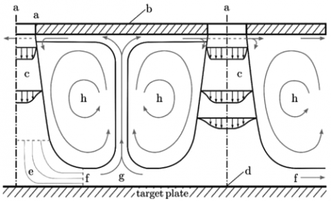
The flow characteristics from multiple impinging jets have regions similar to the flow field from a single impinging jet, however, there are two types of interactions that do not occur in a single impinging jet (see Figure 2). The first is the possible jet interference before impingement onto the target surface. This type of interaction occurs for arrays with very low jet to jet spacings and large nozzle to target surface distances. The second is the interaction due to the collision of surface flows from the adjacent jets, also referred to as secondary stagnation zones. This type of interaction predominantly occurs for arrays with small jet to jet spacing, small jet to surface distance, and large jet velocities. Depending on the strength of this interaction, the fountains can develop between the pairs of adjacent jets and form the recirculating vortices. The above effects can be accentuated further by an additional interaction with the crossflow formed by the spent air of the jets [2].
Figure 2. Complex flow pattern within an impinging jet array [4] a – orifice, b – target plate, c – free jet, d – stagnation point, e – stagnation zone, f – decelerated flow, g – recirculating flow, h – vortices [2]
The heat transfer between an impinging jet and a target surface is affected by many different factors, such as jet exit velocity, velocity profile, turbulence level, entrainment conditions, nozzle geometry, the separation distance between a jet and target surface, the thermal wall boundary conditions, surface motion, and surface curvature. Due to this manifold dependence, the variation of local heat transfer coefficients is very complex.
Figure 3 shows a typical distribution of local heat transfer rates for a single impinging jet along with the target plate. For a single impinging jet, the point of maximum heat transfer is typically the stagnation point (except for very low separation distances), from which the heat transfer rates decrease monotonously in the radial direction. Heat transfer coefficients at the stagnation point increase with the jet Reynolds number. For low separation distances or high jet Reynolds numbers, the secondary peak can appear in the local heat transfer distribution at approximately r/d = 2. There has been a great scientific interest in the origins of the secondary peak. It has been speculated that the secondary peaks are related to the transition from a laminar to a turbulent flow. The heat transfer rates due to the arrays of impinging jets give qualitatively similar results for the single impinging jet, when the jets are widely spaced and, as a consequence of this, no significant jet interaction is present. However, low jet to jet spacing or small jet to surface distance increases the jet interaction and the heat transfer rate changes significantly compared to the single jet. The changes in the heat transfer rate are due to the two types of jet interaction described above [2].
Figure 3. Local Nusselt number distributions along the target plate (Re = 23000, H/d = 2) [6]
5.1 Mathematical formulation
In the following, the conservation laws of mass, momentum, and energy are expressed for an incompressible fluid with the constant fluid properties in steady state form:
$\frac{\partial {{U}_{i}}}{\partial {{X}_{i}}}=0$ (1)
${{U}_{j}}\frac{\partial {{U}_{i}}}{\partial {{X}_{j}}}=\frac{\partial }{\partial {{X}_{j}}}\left( \nu \frac{\partial {{U}_{i}}}{\partial {{X}_{j}}} \right)-\frac{1}{\rho }\frac{\partial P}{\partial {{X}_{j}}}$ (2)
${{U}_{j}}\frac{\partial \Theta }{\partial {{X}_{j}}}=\frac{\partial }{\partial {{X}_{j}}}\left( {{\Gamma }_{\Theta }}\frac{\partial \Theta }{\partial {{X}_{j}}} \right)+{{q}_{\Theta }}$ (3)
The Reynolds-Averaged Navier Stokes equations are solved for the transport of mean flow quantities with appropriate RANS turbulence models to describe the influence of the turbulent quantities to provide closure relations. Each solution variable in the instantaneous Navier-Stokes equations should be decomposed into an averaged value and a fluctuating component to obtain the Reynolds-Averaged Navier-Stokes equations. The resulting equations for the mean quantities are essentially identical to the original equations, except that an additional term now appears in the momentum transport equation. This additional term, known as the Reynolds stress tensor, has the following definition:
${{T}_{t}}=-\overline{{{{{U}'}}_{i}}{{{{U}'}}_{j}}}$ (4)
The challenge is thus to model the Reynolds stress tensor to close the time-averaged equations. Eddy viscosity models employ the concept of a turbulent viscosity for modeling of Reynolds stress tensor. The most common model is known as the Boussinesq approximation:
${{T}_{t}}=2{{\nu }_{t}}{{S}_{ij}}-\frac{2}{3}{{\delta }_{ij}}k$ (5)
where, vt is the turbulent viscosity, k is the turbulence kinetic energy, δij is the Kronecker delta (=1 if i=j, otherwise =0) and Sij is mean strain rate tensor and given by:
${{S}_{ij}}=\frac{1}{2}\left( \frac{\partial {{\overline{U}}_{i}}}{\partial {{X}_{j}}}+\frac{\partial {{\overline{U}}_{j}}}{\partial {{X}_{i}}} \right)$ (6)
Since the assumption that the Reynolds stress tensor is linearly proportional to the mean strain rate and does not consider the anisotropy of turbulence, some two-equation models extend the linear approximation to include the non-linear constitutive relations. The use of hybrid models as a combination of efficient two-equation models is advisable. The Shear Stress Transport (SST) k-ω model as a combination of the k-ε model in the freestream and the standard k-ω model in the inner parts of the boundary layer is an obvious choice.
A Reynolds stress transport (RST) model, also known as the second-moment closure model, calculates all individual components of the Reynolds stress tensor directly by solving their governing transport equations. This type of model is potentially able to predict the complex flows more accurately than the eddy viscosity models, because the transport equations for the Reynolds stresses naturally account for the effects of streamline curvature, swirl rotation, turbulence anisotropy and high rate of strain, but are often unstable when used in the complex flows.
A Large Eddy Simulation (LES) resolves the turbulent structures in space everywhere in the flow domain down to the grid limit, where the subgrid models approximate the impact of the subgrid structures on the flow field. To resolve the crucial turbulent structures near the target wall, this approach requires an excessively high grid resolution in the wall boundary layer: not only in the direction normal to the wall but also in the flow direction. As a result of the high computational costs that go with the high cell count, the LES is used mainly for academic applications or for flows with low Reynolds numbers.
The Hybrid LES-RANS approach resolves the turbulent structures only away from the walls and covers the wall boundary layers by a RANS model. Thereby, the Hybrid LES-RANS avoids the expensive grid requirements of LES. For further details, see [25].
5.2 Domain and boundary condition
Although the impinging jet problem appears simple it is a challenging phenomenon to predict accurately, especially when the nozzle to plate distance is small. The present investigation concentrates on conditions that seem representative of drying applications, i.e. low separation distance and high jet Reynolds number. Among this large variety of experiments, one particular case (Re = 2.3×10⁴, H/d =2) has been investigated in several independent studies. From a large amount of experimental data on this particular configuration, an ERCOFTAC test case was generated. In the present investigation, this case is used due to its good documentation as a benchmark for the evaluation of the turbulence model. Figure 4 shows a schematic of the computational domain for the single impinging jet. Note that this model is based on the assumption of axisymmetry of the problem. In the radial direction, the domain size was 10d, and in the axial direction measured H+2d. These dimensions ensured that the outlet planes were placed at a sufficiently large distance from the region of interest, i.e. the core impingement zone [17].
Figure 4. Computational domain and coordinate system for the single jet cases [17]
The fluid entered the domain with a fully developed turbulent velocity profile obtained from separate computations. For the incoming flow, the turbulence intensity was set to 0.045. The total temperature of the entering fluid was set to a uniform value of Tj=298.15°K. The target plate was modeled as a no-slip wall boundary condition with a constant wall temperature (Tw=330°K). The top and lateral sides of the domain were set to a pressure outlet boundary condition [17].
5.3 Computational details
The numerical model is based on the solution of the stationary Reynolds-averaged Navier-Stokes equation with a finite volume method. This computational fluid dynamics (CFD) model is set up and run with the commercial code STAR-CCM+ 13.02.013 by CD-Adapco [25]. The final solution was obtained by applying a second-order discretization upwind scheme for the pressure, momentum, and energy terms, and the SIMPLE algorithm is used for pressure-velocity coupling and a segregated flow solver was used for all the calculations. The flow in the near-wall regime was simulated using a low-Reynolds number approach which allows the solution of the viscous sublayer using very fine grid length scales next to the wall. The minimum dimensionless wall distance of the first grid node was therefore defined to be always y+≤1. The solution was considered to be converged when the value of the scaled residual of the continuity, momentum, and energy equations is less than 10-4. Convergence is also monitored by plotting the average Nusselt number on the target surface until the variation of the average Nu number levels off with iteration.
5.4 Grid generation and sensitivity
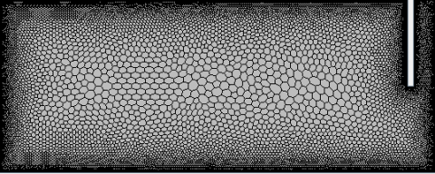
The spatial discretization of the computational domain was realized by an unstructured polygonal grid. STAR-CCM+ produces a real two-dimensional grid from selected two-dimensional part surfaces. Meshing is required to discretize the fluid domain into nodes and volumetric elements so that a fluid flow and heat transfer solution can be obtained for each element. The simple topology of the problem resulted in a grid with a total cell number of approximately 40579 (see Table 1). The resulting grid is shown in Figure 5. The majority of cells were concentrated along the wall boundary to account for the development of the wall jet boundary layer.
Table 1. Grid parameters used for the grid sensitivity analysis
|
Grid |
Base size(mm) |
Cell number |
$\mathrm{y}_{1, \max }^{+}$ |
Average GCI % |
|
Coarse |
2.0 |
8862 |
0.22 |
--- |
|
Intermediate |
1.0 |
19143 |
0.11 |
0.63 |
|
Fine |
0.5 |
40579 |
0.087 |
0.26 |
Figure 5. Two-dimensional view on an unstructured polyhedral grid
Figure 6. Nusselt number distributions obtained by the grids used in the grid sensitivity study
For a quantification of the discretization error, the benchmark case (H/d=2, Re=23000) was taken. The grid sizes are summarized in Table 1 indicating that the y1+ requirement was fulfilled for all investigated grids. Here, $y_{1, \max }^{+} \leq 1$ refers to the maximum value of the dimensionless distance between the target plate and the first node. The base size specifies the reference length value for all relative size control. The Nusselt number distributions obtained by the different grids are shown in Figure 6. Note that due to the symmetry of the problem, only half of the target plate is shown. The local discretization error distribution is calculated by applying the Grid Convergence Index (GCI) method [26] to the y-centerline Nu distribution. The overall discretization error for fine and intermediate grids was very small (average 0.26% and 0.63% respectively). However, in the present case, the solution was grid-independent so that the results of the different grids were as good as identical. To reduce the computational cost, the intermediate grid is selected as the final grid.
6.1 Evaluation of computational model
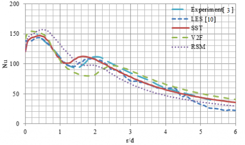
Figure 7 shows a typical distribution of the local Nu number for a single impinging jet along with the target plate (Re =23,000, H/d = 2). As shown in Figure 7, the local Nusselt numbers increase from the stagnation point toward the primary peak at 0.5 nozzle diameter (r/d~0.5) and then decrease rapidly to reach local minima and again increase along the wall, giving the second peak in the transition region at approximately r/d= 2. Moving outward from the secondary peak, the heat transfer rates decrease monotonically into the wall jet region. There has been a great scientific interest in the origins of the secondary peak. It has been speculated that the formation of the secondary maxima is related to the increased momentum transport due to the transition from a laminar to a turbulent boundary layer. Baughn et al. [3] gave similar results but did not show the first peak. This may be attributed to the lower spatial resolution in the stagnation region compared with the present study. The CFD results show that the main characteristics of the heat transfer pattern, i.e. stagnation point, primary peaks, and secondary peaks, are adequately reproduced. The heat transfer level agrees very well for the stagnation point, primary and secondary peaks. SST turbulence model can predict the strong shape of primary and secondary peaks of Nu number. Although the SST turbulence model from this work predicted the strong shape of the secondary peak, it was mismatched in position. However, the secondary peak was not represented correctly by other implementations of the SST model as shown in the literature (see Figure 7).
Figure 7. Local Nu number distributions predicted by STAR CCM+ in comparison to the experimental and numerical results from the literature
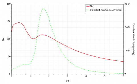
Figure 8 shows the Nusselt number and turbulent kinetic energy distributions of jet impingement flow near the wall region. The location of the primary and secondary peak of turbulent kinetic energy is a coincidence with the location of the primary and secondary peak of Nu number. That’s why the accuracy of the Nusselt number computation correlates with the quality of the turbulence model used. This numerically predicted effect correlates well with the findings of [7, 8] who suggested that the location of the secondary peak coincided with the point where the turbulent kinetic energy became the maximum.
Figure 8. Nu number and turbulent kinetic energy distributions of jet impingement flow near the wall region
6.2 Distribution of Nusselt number
The Nusselt number distribution especially the secondary peak is strongly influenced by the turbulence model used. The scope of this research is to investigate the possible factors on the origin of this behavior in more detail such as the effect of different turbulence models, transition models, grid shape, and grid size.
6.2.1 Turbulence models
The choice of turbulence model is of fundamental importance for an accurate numerical simulation of jet impingement heat transfer, as the resulting heat transfer rates are directly depending on the predicted flow and turbulence characteristics. From the available models in STAR-CCM+, different models were tested including eddy-viscosity models and models of the second-order closure type. This selection represents the most commonly used groups of turbulence models for engineering applications in turbomachinery. As representatives for various types of RANS models; V2F, SST, and Reynolds stress models were included, due to the recommendation of the researcher in the literature. For the analysis of the flow structures, a LES or DNS is preferable, as these kinds of simulations are possible with the increasing computational power available, as well as the advance in the use of efficient and higher-order numerical schemes. The result of LES and also the experimental result are extracted from literature for comparison with numerical simulations (Figure 9).
Examination of RANS numerical modeling techniques showed that the various implementations of the V2F and RSM models give large errors compared to the experimental data. The computational times will vary with model complexity and computing power. In comparison, the RSM and V2F could need more computational times (around 53% and 40% respectively) and memory requirement (around 10% and 4% respectively) than SST (see Table 2). Giovannini and Kim [19] stated that a well-resolved three-dimensional LES impinging jet model could take a day to provide a solution. On the other hand, the SST turbulence model predicted the strong shape of the primary and secondary peak of local Nusselt number distributions better than other models and is recommended as the best compromise between solution speed and accuracy and also this correlates well with the findings of Badra et al. [14] who found that the SST k–ω turbulence models succeeded with reasonable accuracy (within 20% error) in reproducing the experimental data and the second peak in the local Nu number at the low jet to surface distances was well predicted by the SST k–ω model.
Figure 9. Local Nusselt number distributions predicted by different turbulence models in comparison to experimental data
Table 2. Total solver CPU time and memory requirement for different turbulence model
|
Turbulence model |
Total solver CPU time (s) |
Memory requirement (KB) |
|
RSM |
168 |
6.112 |
|
V2F |
154 |
5.691 |
|
SST |
110 |
5.484 |
6.2.2 Transition model
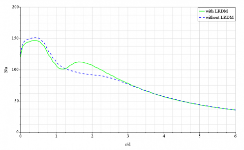
Since the secondary peak is related to the transition of the flow from laminar to turbulent, the prediction of the secondary peak might be enhanced by using a transition model in combination with the turbulence model. The low-Reynolds number modification can be used to account for the low-Reynolds number and transitional effects.
Figure 10. Effect of low Re damping modification in the prediction of local Nu number
Figure 10 indicates the effect of low Re damping modification in the prediction of local Nu number distribution. This modification has an important role in the prediction of location and intensity of secondary peak and therefore this is a most important reason for better prediction of present research in comparison with other CFD simulations such as Spring 2010 [17] who did not use a transition model in combination with a turbulence model (see Figure 7).
6.2.3 Grid shape
Researchers have usually used the hexahedral grid and no investigation with regard to the effect of other grid shapes in the prediction of the secondary peak was observed. To investigate this matter, three different unstructured grid shapes (tetrahedral, hexahedral, and polyhedral) are considered. A two-dimensional view on these grids is shown in Figure 11.
Figure 12 indicates the effect of grid shape in the local Nusselt number distribution. No significant change was observed in the prediction of position and intensity of the Nu number at the primary and secondary peak for different grid shapes, in contrast, the Nu number at the stagnation point was very sensitive to the grid shape.
It is very important to investigate the effect of grid shape for the coarse grid equal to approximately 8000 cells. Figure 13 indicates the result of this investigation. There is no difference for different grid shapes in the prediction of the secondary peak, but the hexahedral and tetrahedral grids cannot predict the strong shape of the primary peak as accurately as of the polyhedral grid. Moreover, the stagnation point still has the sensitivity to the grid shape similar to the intermediate grid.
Table 3 shows the total solver CPU time and memory requirement for different grid shapes. The polyhedral grid requires less computational memory and cell number and provides faster post-processing time compared to two other grid shapes. The results, therefore, demonstrate the ability of the polyhedral grid to produce good quality results with lower memory requirement and shorter run times than other grid types and there is a minor difference in the quality of the results from the three grids at the primary and secondary peaks, although there is a significant difference between three grids at the stagnation point.
Table 3. Total solver CPU time and memory requirement for different grid shapes
|
Grid shape |
Cell number |
Total solver CPU time (s) |
Memory requirement (MB) |
|
Polyhedral |
19143 |
111 |
175.33 |
|
Tetrahedral |
25380 |
224 |
172.72 |
|
Hexahedral |
25429 |
318 |
190.05 |
Figure 11. Two-dimensional view on different grid shapes
Figure 12. Effect of grid shape in the prediction of the Nu number distribution for intermediate grid
6.2.4 Grid size
It is very important to investigate the grid size and amount of deviation in the prediction of secondary peak related to a very fine grid as the exact solution. Table 4 shows the grid size in conjunction with the position and intensity of the Nu number at the stagnation point, primary peak, and secondary peak. The base size=0.1mm is considered as very fine grid and a reference for deviation of other coarser grids. The $y_{1, \max }^{+} \leq 1$ requirement was fulfilled for all investigated grids.
Figure 13. Effect of grid shape in the prediction of the Nu number distribution for coarse grid
Table 4. Grid parameters used for the deviation analysis
|
Total solver CPU time(s) |
Secondary peak r/d Nu |
Primary peak r/d Nu |
Stagnation point r/d Nu |
Cell number |
Base size (mm) |
|||
|
25 |
103.203 |
1.62 |
-- |
-- |
180.125 |
0.0 |
5695 |
3.0 |
|
32 |
108.6 |
1.62 |
149.032 |
0.42 |
165.5 |
0.0 |
6932 |
2.5 |
|
41 |
110.33 |
1.62 |
149.83 |
0.36 |
116.955 |
0.0 |
8862 |
2.0 |
|
111 |
112.5 |
1.62 |
147.0 |
0.42 |
120.7 |
0.0 |
19143 |
1.0 |
|
326 |
113.07 |
1.68 |
146.02 |
0.42 |
137.231 |
0.0 |
40579 |
0.5 |
|
954 |
112.9 |
1.68 |
145.30 |
0.48 |
144.018 |
0.0 |
84770 |
0.25 |
|
3927 |
111.5 |
1.68 |
145.34 |
0.48 |
142.4 |
0.0 |
220713 |
0.1 |
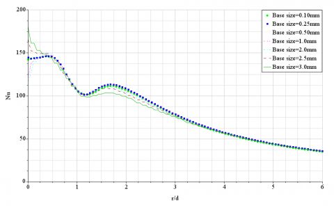
Figure 14. Effect of grid size in the prediction of local Nu number distribution
Figure 14 shows the effect of grid size in the prediction of local Nu number distribution. The relative deviation of Nu number value for coarse grids up to base size=2mm related to the reference grid at the primary peak, secondary peak, and the stagnation point is approximately 1.18%, 1.15%, and 11.12% in average respectively. The relative deviation of Nu number location for coarse grids up to base size=2mm related to the reference grid at the primary peak, secondary peak, and the stagnation point is approximately 12.5%, 0.0% and 0.0% in average respectively. It can be concluded from Table 4 and Figure 14 that the coarse grids up to base size=2mm can succeed to predict the location and intensity of Nu number at the stagnation point, primary and secondary peaks with a reasonable level and very lower computation time compared to the very fine grid.
In this paper, the single impinging jet for symmetric configuration (2D) is considered. For the problem, a computational model was generated to represent the experimental investigations used as a reference. Using a particular configuration (Re=2.3×10⁴, H/d=2), for which several independent sources of experimental data exist, the predictions from different turbulence models were analyzed. The findings of this investigation are as follows:
It can be concluded from the evaluation of different turbulence models with regards to predictions of heat transfer that the SST turbulence model represents a good compromise between the accuracy of its results and the computational effort. Although the SST turbulence model from literature was not represented correctly the secondary peak, the SST turbulence model from this work predicted the strong shape of the secondary peak, it was mismatched in position. Low Re damping modification in implementation of SST K-ω has an important role in the prediction of location and intensity of the secondary peak. Good results can be achieved with a coarse grid to predict the position and intensity of Nu number at the stagnation point, primary and secondary peaks with a reasonable level, and very lower computation time compared to very fine grids, as long as the boundary region is appropriately resolved. The results demonstrate the ability of polyhedral grids to produce good quality results with lower memory requirement and cell number as well as shorter run times than other grid shapes and there is little difference in the quality of the results from other grids, although the result from the polyhedral grid is slightly better than the other two in the stagnation point.
|
d |
nozzle diameter, m |
|
H |
nozzle to plate distance, m |
|
h |
heat transfer coefficient, W/m2K |
|
i, j, k |
tensor indices |
|
k |
turbulence kinetic energy, J/kg |
|
kt |
thermal conductivity, W/mK |
|
Nu |
local Nusselt number (hd/kt) |
|
P |
pressure, Pa |
|
r |
radial coordinate on the surface, m |
|
Re |
Reynolds number, $\bar{U} \mathrm{~d} / \mathrm{v}$ |
|
T |
temperature, K |
|
Tt |
Reynolds stress tensor |
|
U |
velocity, m/s |
|
$\bar{U}$ |
average velocity, m/s |
|
Ui |
instantaneous components of the velocity vector in the direction Xi, m/s |
|
$U_{i}^{\prime}$ |
fluctuating components of the velocity vector in the direction Xi, m/s |
|
x, y |
coordinates |
|
y+ |
dimensionless wall distance |
|
Abbreviation |
|
|
CFD |
computational fluid dynamic |
|
CPU |
central processing unit |
|
DNS |
direct numerical simulation |
|
GCI |
grid convergence index |
|
LES |
large eddy simulation |
|
LRDM |
low Re damping modification |
|
RANS |
Reynolds-average Navier-stokes |
|
RSM |
Reynolds stress model |
|
SST |
shear stress transport |
|
Greeks |
|
|
ν |
kinematic viscosity, m2/s |
|
νt |
turbulent viscosity, m2/s |
|
ԑ |
dissipation rate, m2/s3 |
|
ω |
specific dissipation rate, 1/s |
|
ρ |
density, kg/m3 |
|
δij |
Kronecker delta |
|
Sij |
mean strain rate tensor, m/s2 |
|
Θ |
general scalar variable |
|
$\Gamma_{\Theta}$ |
diffusivity of Θ, m2/s |
|
Subscripts |
|
|
j |
jet |
|
w |
wall |
[1] Nastase, I., Bode, F. (2018) Impinging jets – A short review on strategies for heat transfer enhancement. E3S Web of Conferences, 32: 01013. https://doi.org/10.1051/e3sconf/20183201013
[2] Weigand, B., Spring, S. (2011). Multiple jet impingement−A review. J. Heat Transfer Research, 42: 101-142. http://doi.org/10.1615/HeatTransRes.v42.i2.30
[3] Baughn, J., Hechanova, A., Yan, X. (1991). An experimental study of entrainment effects on the heat transfer from a flat surface to a heated circular impinging jet. J. Heat Transfer, 113(4): 1023-1025. https://doi.org/10.1115/1.2911197
[4] Patil, V.S., Vedula, R.P. (2018). Local heat transfer for jet impingement on a concave surface including injection nozzle length to diameter and curvature ratio effects. J. Experimental Thermal and Fluid Science, 92: 375-389. https://doi.org/10.1016/j.expthermflusci.2017.08.002
[5] Lytle, D., Webb, B.W. (1994). Air jet impingement heat transfer at low nozzle-plate spacings. Int. J. Heat and Mass Transfer, 37: 1687-1697. https://doi.org/10.1016/0017-9310(94)90059-0
[6] Katti, V., Prabhu, S.V. (2008). Experimental study and theoretical analysis of local heat transfer distribution between smooth flat surface and impinging air jet from a circular straight pipe nozzle. International Journal of Heat and Mass Transfer, 51(17-18): 4480-4495. https://doi.org/10.1016/j.ijheatmasstransfer.2007.12.024
[7] Den Ouden, C., Hoogendoorn, C.J. (1974). Local convective-heat-transfer coefficients for jets impinging on a plate; Experiments using a liquid-crystal technique. In Heat transfer; Proceedings of the Fifth International Conference, Tokyo, 5: 293-297. https://doi.org/10.1615/ihtc5.2770
[8] Narayanan, V., Seyed-Yagoobi, J., Page, R.H. (2004). An experimental study of fluid mechanics and heat transfer in an impinging slot jet flow. International Journal of Heat and Mass Transfer, 47: 1827-1845. https://doi.org/10.1016/j.ijheatmasstransfer.2003.10.029
[9] Kataoka, K., Suguro, M., Degawa, H., Maruo, K., Mihata, I. (1987). The effect of surface renewal due to largescale eddies on jet impingement heat transfer. International Journal of Heat and Mass Transfer, 30: 559-567. https://doi.org/10.1016/0017-9310(87)90270-5
[10] Uddin, N., Neumann, S.O., Weigand, B. (2013). LES simulations of an impinging jet: On the origin of the second peak in the Nusselt number distribution. Int. J. Heat and Mass Transfer, 57(1): 356-368. https://doi.org/10.1016/j.ijheatmasstransfer.2012.10.052
[11] Choi, M., Yoo, H.S., Yang, G., Lee, J.S., Sohn, D.K. (2000). Measurements of impinging jet flow and heat transfer on a semi-circular concave surface. Int. J. Heat and Mass Transfer, 43(10): 1811-1822. https://doi.org/10.1016/S0017-9310(99)00257-4
[12] Yan, W.M., Liu, H.C., Soong, C.Y. (2003). Experimental study of impinging heat transfer of inline and staggered jet arrays by transient liquid crystal technique. J. Flow Visualization and Image Processing, 10: 1-2. http://doi.org/10.1615/JFlowVisImageProc.v10.i12.70
[13] Wae-Hayee, M., Tekasakul, P., Eiamsa-Ard, S., Nuntadusit, C. (2015). Flow and heat transfer characteristics of in-line impinging jets with cross-flow at short jet-to-plate distance. J. Experimental Heat Transfer, 28(6): 511-530. https://doi.org/10.1080/08916152.2014.913091
[14] Badra, J., Masri, A.R., Behnia, M. (2013). Enhanced transient heat transfer from arrays of jets impinging on a moving plate. J. Heat Transfer Engineering, 34(4): 361-371. https://doi.org/10.1080/01457632.2013.717046
[15] Sharif, M.A.R., Mothe, K.K. (2009). Evaluation of turbulence models in the prediction of heat transfer due to slot jet impingement on plane and concave surfaces. J. Numerical Heat Transfer, Part B: Fundamentals, 55(4): 273-294. https://doi.org/10.1080/10407790902724602
[16] Yang, B., Chang, S., Wu, H., Zhao, Y., Leng, M., (2017). Experimental and numerical investigation of heat transfer in an array of impingement jets on a concave surface. J. Applied Thermal Engineering, 127: 473-483. https://doi.org/10.1016/j.applthermaleng.2017.07.190
[17] Spring, S. (2010). Numerical prediction of jet impingement heat transfer. Ph.D. Thesis, Faculty of Aerospace Engineering and Geodesy, Universität Stuttgart.
[18] Benhacine, A., Kharoua, N., Khezzar, L., Nemouchi, Z. (2012). Large eddy simulation of a slot jet impinging on a convex surface. International Journal of Heat and Mass Transfer, 48(1): 1-15. https://doi.org/10.1007/s00231-011-0835-3
[19] Giovannini, A., Kim, N.S. (2006). Impinging jet: Experimental analysis of flow field and heat transfer for assessment of turbulence models. Proceedings of 13th International Heat Transfer Conference, Sydney, Australia. http://doi.org/10.1615/IHTC13.p1.150
[20] Penumadu, P.S., Rao, A.G. (2017). Numerical investigations of heat transfer and pressure drop characteristics in multiple jet impingement system. J. Applied Thermal Engineering, 110: 1511-1524. https://doi.org/10.1016/j.applthermaleng.2016.09.057
[21] Wilke, R., Sesterhenn, J. (2015). Direct numerical simulation of heat transfer of a round subsonic impinging jet. In Active Flow and Combustion Control, 127: 147-159. https://doi.org/10.1007/978-3-319-11967-0_10
[22] Cooper, D., Jackson, D.C., Launder, B.E., Liao, G.X. (1993). Impinging jet studies for turbulence model assessment—I. Flow-field experiments. International Journal of Heat and Mass Transfer, 36(10): 2675-2684. https://doi.org/10.1016/S0017-9310(05)80204-2
[23] Penumadu, P.S., Rao, A.G. (2017). Numerical investigations of heat transfer and pressure drop characteristics in multiple jet impingement system. J. Applied Thermal Engineering, 110: 1511-1524. https://doi.org/10.1016/j.applthermaleng.2016.09.057
[24] Kubacki, S., Dick, E. (2011). Hybrid RANS/LES of flow and heat transfer in round impinging jets. Int. J. Heat and Fluid Flow, 32: 631-651. https://doi.org/10.1016/j.ijheatfluidflow.2011.03.002
[25] STAR-CCM+ 13.02.013 User Guide by CD-Adapco.
[26] Roache, P.J. (2003). Conservatism of the grid convergence index in finite volume computations on steady-state fluid flow and heat transfer. J. Fluids Engineering, 125: 731-732. https://doi.org/10.1115/1.1588692