Xiaogai Shen
© 2021 IIETA. This article is published by IIETA and is licensed under the CC BY 4.0 license (http://creativecommons.org/licenses/by/4.0/).
OPEN ACCESS
Establishing and optimizing an integrated central heating information monitoring and energy conservation system can not only help reduce the waste of resources, but also allow us to identify and solve the instability and safety problems in the heating process, and thus this system is of certain research value. Existing automated heating equipment fail to truly monitor and regulate heating due to various reasons like the lack of comprehensive parameter measurement and serious hydraulic imbalance of the system. To this end, this paper studies the design and implementation of an integrated central heating information monitoring system for smart cities. First, the big data of central heating temperature monitoring in smart cities was reconstructed, and then three different central heating regulation modes were introduced. The experimental results verified the effectiveness of the proposed algorithm. With an example of central heating monitoring shown, the energy efficiency analysis results regarding the energy conservation optimization of the system were given.
central heating, information monitoring, big data reconstruction, heating regulation mode
In the process of extensive economic development, the energy consumption in China has been increasing year by year, with the total energy consumption being much higher than the world average, and the case is the same with heat consumption [1-6]. Due to the geographical dispersion of urban heat supply, the central heating system is required to monitor and analyze parameters such as thermal energy, heating power and heat supplied, etc., to further realize the linkage between heat dispatching and heat exchange stations [7-14]. Establishing and optimizing an integrated central heating information monitoring and energy conservation system is not only conducive to reducing resource waste, but also helpful to the identification and solving of the instability and safety problems in the heating process, and thus it has certain research value.
The central heating technology has a development history of nearly a hundred years, and thus there has been in-depth research on heating at home and abroad. Liu [15] conducted the energy conservation analysis and comprehensive energy efficiency evaluation of a campus central heating system based on the heating monitoring platform, elaborated the energy consumption analysis method for the campus central heating system based on the heating monitoring platform, and gave the energy balance equation. Schuetz et al. [16] adjusted the parameters in the simplified physical simulation model of the building and heating system to match the simulation and actual power consumption of the heat pump. Parhizkar et al. [17] proposed that the central heating system should select sensors based on the priority of sensors in providing system health information. Based on the Bayesian network model, it optimized the sensor types that consider the correlation of faults between components, and applied the proposed method to a central heating system as a case study. Burgas et al. [18] proposed a method for monitoring building heating systems based on principal component analysis. The proposed method allows the definition of simple statistical indexes T2 and SPE for monitoring graphs and detecting abnormal behaviors and also for controlling heating systems. Pippia et al. [19] proposed combining the MPC controller based on random scenarios with the nonlinear Modelica model. The proposed model can provide a richer building description and capture the building dynamics more accurately than the linear model.
At present, the domestic central heating management mainly relies on manual regulation and control based on operators’ experience. The advanced automation equipment installed fail to truly monitor and regulate heating due to various reasons such as lack of comprehensive parameter measurement, serious hydraulic imbalance of the system, mismatch between heat supply and heat demand, and huge sizes of thermal and hydraulic parameters. For this reason, this paper conducts research on the design and implementation of an integrated central heating information monitoring system for smart cities. Section 2 of this paper first reconstructs the big data of central heating temperature monitoring in smart cities, and elaborates on the principle of reconstruction, the steps to establish the compressed sensing measurement matrix, and the steps to reconstruct central heating temperature monitoring data; Section 3 introduces the three different central heating regulation modes, namely the heating quality regulation mode, the heating flow regulation mode, and the staged integrated heating regulation mode. The experimental results verify the effectiveness of the proposed algorithm. With an example of central heating monitoring shown, the energy efficiency analysis results regarding the energy conservation optimization of the system were given.
2.1 Principle of reconstruction
Figure 1 shows the structure of the integrated central heating information monitoring system for smart cities. The system realizes informatization of heating and management and control mainly through information management functions like pipeline planning, maintenance management, equipment management, configuration software functions like heat meter reading, hydraulic analysis, balance adjustment, data acquisition control and heating data mining and also system administration functions provided for operators like human-machine interfaces and heating regulation and energy-conservation optimization plan reading. In the chart, the data acquisition control module of the integrated central heating information monitoring system for smart cities conducts real-time monitoring of the temperature indicator in each target heating area through various temperature sensor terminals, and transmits the massive temperature monitoring data through the wireless network data transmission system to the base station of the integrated monitoring system for subsequent data mining and analysis.
With the number of central heating users increasing in cities, the volume of real-time heating data is getting larger and larger, and the limitations of the traditional data mining and analysis technologies are gradually showing. Nyquist sampling, which is often used in the traditional data compression technology, requires a sufficiently high sampling rate of the sampling device, resulting in the high cost of the device.
Figure 1. Structure chart of the integrated central heating information monitoring system
Figure 2. Schematic diagram of compressed sensing sampling
Figure 3. Block diagram of the sparsity adaptive matching pursuit algorithm
Considering that compressed sensing can improve the problems of the traditional technology such as low processing efficiency, insufficient resource utilization, and high information redundancy, this paper used this technology to process massive heating information to reduce the hardware requirements in the storage and transmission process of heating information and control signals. Figure 2 shows the schematic diagram of compressed sensing sampling. It can be seen that under the premise that the central heating temperature monitoring data are sparse, the data can be sparsely represented and sampled at a low speed, and after data dimension reduction, the reconstructed values can be obtained.
Considering the application scenarios of central heating temperature monitoring, this paper made some improvement to the greedy algorithm, which is widely applied in compressed sensing, to realize accurate reconstruction of the grid data of central heating temperature monitoring.
Figure 3 shows the block diagram of the sparsity adaptive matching pursuit algorithm. Based on this algorithm, this paper introduces the threshold method of the stagewise orthogonal matching pursuit algorithm, and proposes a threshold-based sparsity adaptive matching pursuit algorithm, which is applicable to the situation where there is no need to obtain the sparsity of the acquired central heating information in advance. The algorithm consists of the following 5 steps:
Step1: Initialize the residual s0, the index set Γ0 and the step size K:
$s_{0}=b, \Gamma_{0}=\psi, K=e$ (1)
Step2: In order to select the most relevant index set, calculate the inner product of the sensing matrix C and the residual s using Eq. (2):
$v=IP\left[ {{C}^{T}}{{s}_{\tau -1}} \right]$ (2)
Step3: Obtain the candidate atom set Dl and the column set Cτ shown in Eq. (3) based on the threshold method:
${{D}_{l}}={{\Gamma }_{\tau -1}}\bigcup {{E}_{l}}\bigcup {{I}_{0}},{{C}_{\tau }}=\left\{ {{c}_{i}} \right\}\left( i\in {{D}_{l}} \right)$ (3)
Step4: Based on the two sets Dl and Cτ, use the least square method to solve the estimated value of the central heating temperature data ω, and select the K term with the largest inner product value v:
${{\dot{\omega }}_{\tau }}=arg\underset{\omega }{\mathop{min}}\,\left\| b-{{C}_{\tau }}{{\omega }_{\tau }} \right\|={{\left( C_{\tau }^{T}{{C}_{\tau }} \right)}^{-1}}C_{\tau }^{T}b$ (4)
Step5: Update the support set CτK, and further update the residual according to Eq. (5):
$s_{N}=b-C_{\tau K}\left(C_{\tau K}^{T} C_{\tau K}\right)^{-1} C_{\tau K}^{T} b$ (5)
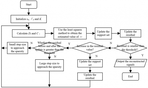
Figure 4. Flow chart of the improved threshold-based algorithm
Check whether the updated residual value is smaller than a preset threshold. If it is smaller than the preset value, output the reconstructed signals and end the iteration. If it is greater, make a further judgment on whether the residual value is increased. If the residual value is increased and at the same time, the residual before and after the update is greater than the preset threshold, then enter the stage of large step size to approach the sparsity, and if it is not, enter the stage of small step size to approach the sparsity. If the residual value is decreased, update the support set and the residual before returning to the iteration. Figure 4 shows the flow chart of the improved threshold-based algorithm.
2.2 Establishment of the compressed sensing measurement matrix
In the compressed sensing theory, the compressed sensing measurement matrix, which is mainly used for data dimension reduction, has an important effect on the reconstruction effect of the central heating temperature monitoring data. Considering the specificity of the grid data of central heating temperature monitoring, the data characteristics need to be effectively extracted and used on the basis of the classic measurement matrix to achieve the best data reconstruction effect. The basic principle of the compressed sensing measurement matrix used in this paper is described as follows:
Since the compressed sensing measurement matrix needs to satisfy the restricted isometry property, the parameter ξl with the finite equidistance property should be first defined. Eq. (6) gives the inequality that the minimum value ξ needs to satisfy:
$(1-\xi)\|a\|_{2}^{2} \leq\|\Psi a\|_{2}^{2} \leq(1+\xi)\|a\|_{2}^{2}$ (6)
In Eq. (6), a is the finite-duration signal of central heating temperature monitoring with at most L non-zero elements. If ξl<1, it will be deemed that the measurement matrix satisfies the L-order finite equidistance property.
It is difficult to determine whether a measurement matrix meets the finite equidistance property. The irrelevance principle that characterizes the irrelevance between the measurement matrix and the sparse matrix can be used as an equivalent of the finite equidistant property. Assuming that the row vector of the measurement matrix Ψ and the column vector of the sparse basis γ are denoted as Ψi and γj, respectively, the coherence coefficient is expressed as:
$\lambda(\Psi, \gamma)=\sqrt{M} \max _{i, j} \frac{\left|\left(\Psi_{i}, \gamma_{j}\right)\right|}{\left\|\Psi_{i}\right\|_{2}\left\|\gamma_{j}\right\|_{2}}$ (7)
It can be seen from the above equation that the smaller λ is, the more irrelevant Ψ and γ are to each other, and the better the reconstruction effect of the sensing matrix is. Assuming that φ is a certain positive constant, the number of measurements N needs to satisfy the inequality N≥φλ2Llog(M) to ensure that a can be completely reconstructed.
The empirical mode decomposition (EMD) algorithm can carry out decomposition according to the characteristics of the data, which is most applicable to the processing of nonlinear and non-stationary signals. The EMD algorithm can decompose a central heating temperature monitoring signal into multiple independent intrinsic mode components and a residual component based on the data characteristics. The specific decomposition takes the following 5 steps:
Step1: Define the original temporal sequence of central heating temperature monitoring data as a(τ), and extract all the maximum and minimum points in the sequence.
Step2: Use the cubic spline interpolation method to curve fit all the maximum and minimum points in the temporal sequence to generate the upper envelope ENmax(τ) and the lower envelope ENmin(τ).
Step3: Calculate the mean value EN(t) of ENmax(τ) and ENmin(τ) according to Eq. (8):
$E N(\tau)=\frac{E N_{\max }\quad(\tau)+E N_{\min }\quad(\tau)}{2}$ (8)
Step4: Calculate the difference between a(τ) and EN(τ), and the residual signal RS1(τ) is given by Eq. (9):
$R{{S}_{1}}\left( \tau \right)=a\left( \tau \right)-EN\left( \tau \right)$ (9)
Step5: Determine whether RS1(τ) satisfies the constraint conditions for the intrinsic mode components, that is, the number of extreme points must be equal to that of zero-crossing points, and at the same time, the mean value of the upper envelope ENmax(τ) and the lower envelope ENmin(τ) is 0. If the conditions are not satisfied, take RS1(τ) as the new temporal sequence. If the conditions are satisfied, record RS1(τ) as the first intrinsic mode component, and subtract all intrinsic mode components from the original sequence and the remaining part will be the residual component s(τ)=a(τ)-RS(τ) as the new temporal sequence.
Step6: Repeat Step1~Step5 to obtain a new series of intrinsic mode components until the residual component s(τ) is a constant or monotonic function, and the empirical mode decomposition stops.
Assuming that the number of intrinsic mode components is m, the empirical mode decomposition process of the central heating temperature monitoring signal is expressed in Eq. (10):
$a\left( \tau \right)=\sum\nolimits_{i=1}^{m}{R{{S}_{i}}\left( \tau \right)}+s\left( \tau \right)$ (10)
Assuming that the i-th intrinsic mode component is denoted as RSi(τ)=[ui1ui2…uiM-1uiM], and that the length of the original temporal sequence of central heating temperature monitoring signal is denoted as M, the m intrinsic mode components constitute the EMD measurement matrix:
$\left[\begin{array}{llll}u_{1}^{1} & u_{2}^{1} & u_{M-1}^{1} & u_{M}^{1} \\ u_{1}^{2} & u_{2}^{2} & u_{M-1}^{2} & u_{M}^{2} \\\\ u_{1}^{m} & u_{2}^{m} & u_{N-1}^{m} & u_{M}^{m}\end{array}\right]$ (11)
If m is greater than the number of measurements N, the matrix can be constructed based on the first N components. If m is smaller than N, the measurement matrix needs to be expanded to N*M dimensions. The remaining N-m rows are obtained through cyclic shift of the existing m intrinsic mode components.
2.3 Steps to reconstruct the monitoring data of central heating temperature
The compressed sensing technology can effectively reduce the volume of data that need to be transmitted by the central heating temperature monitoring nodes, thereby reducing the power consumption of the integrated monitoring system. Assuming that the N×M-dimensional matrix that meets the finite equidistant property is denoted as D, that the central heating monitoring node location selection matrix as O, and that the overall thermal environment data of the central heating monitoring area after gridding as a, the central heating temperature monitoring data sampling model used in this paper is given in Eq. (12):
$b=DOa=\Psi a$ (12)
The temperature sensors in the central heating temperature monitoring area are randomly placed, and O can characterize the locations of the temperature sensors. If the element in the matrix is 1, it indicates that there is a sensor in the corresponding monitoring area grid. If it is 0, there is no sensor. Assuming that the sensor data vector is represented by a*, Eq. (13) gives the relationship between a, O, and a*:
$a'=Oa$ (13)
The steps of the grid data reconstruction algorithm designed in this paper are listed as follows:
Step1: Designate the central heating temperature monitoring area, arrange temperature sensor nodes in the area that requires temperature monitoring, perform grid processing of the obtained heating monitoring data, and set the area with no temperature sensor to zero;
Step2: Construct the location selection matrix O that records the location of each sensor node;
Step3: Perform spatial interpolation operation on the temperature sensor monitoring data, and then perform empirical mode decomposition on the obtained sensor data vector ai, and multiply D by O to obtain the measurement matrix Ψ;
Step4: Multiply ai by Ψ to get the measured value b, and then use the threshold-based sparsity adaptive matching tracking algorithm to reconstruct the central heating temperature monitoring data to obtain the reconstructed value a*;
Step5: Calculate the structural similarity between a and a*, set the relevant threshold conditions based on the calculation results. If the conditions are not satisfied, repeat the above steps, and if they are, stop the algorithm.
The integrated central heating information monitoring system for smart cities automatically balances the heat distribution of each heat exchange station based on the actual temperature of the heating site and the grid data reconstruction results, to further achieve heat balance of the entire network. This will effectively solve the problem of hydraulic imbalance in the heating system, and save energy and reduce consumption.
The integrated central heating information monitoring system automatically balances the heat distribution of each heat exchange station based on such control parameters as the size of the heating area, the outdoor temperature, and the heat losses of the pipe network and of the buildings. The weighted average scheduling method for heat energy is described in detail as follows.
Suppose that the total heat load of the heating design is denoted as W, that the building area of the heating design as R, and that the heat load per square meter of building area of the heating design as w, which is the heating index of the heating area. Eq. (14) shows the calculation formula for the heat load of the heated building:
$W=w\cdot R/100$ (14)
Let the heat transfer coefficient of the building facade be represented by HTC, the heat transfer area of the building facade HTA, the indoor temperature εm, and the outdoor design temperature εq. w and the basic heat consumption of the building together affect the heat load, and the relationship between the two is expressed by Eq. (15):
$w=\sum{\frac{HTC\cdot HTA\cdot \left( {{\varepsilon }_{m}}-{{\varepsilon }_{q}} \right)}{R}}$ (15)
It can be seen from the above analysis that there is a linear relationship between W and εq. It is defined that between the supply and return water temperature difference of the primary network of the central heating system is equal to the difference between the temperatures of the supply water and the return water in the primary network; and that the supply and return water temperature difference of the secondary network is equal to the difference between the temperature of the supply water and the return water in the secondary network. Assuming that the specific heat capacity is represented by σ and that the water quality by Z, Eq. (16) gives the heat absorption formula:
${{W}_{DE}}=\sigma Z\Delta \varepsilon =\sigma Z\left( {{\varepsilon }_{S}}-{{\varepsilon }_{R}} \right)$ (16)
Eq. (17) gives the heat release formula:
${{W}_{HR}}=\sigma Z\Delta \varepsilon =\sigma Z\left( \varepsilon -{{\varepsilon }_{0}} \right)$ (17)
The heat supply regulation of the integrated central heating information monitoring system for smart cities is the regulation of heat production, transmission and distribution and use according to needs based on the temperature monitoring data. When the heat load changes, the hot water flow pressure in the heating pipe network will change frequently. In order to ensure the on-demand heat supply, a temperature and pressure difference control device needs to be installed to regulate the hydraulic balance in the pipe network.
Let the heat load of the heating design of the building be denoted as W1*, the calculated outdoor heating temperature as εq*, and the heat released by the radiator at εq* and the heat delivered by the hot water network to the residents as W2* and W3*. Let the heating index per unit volume of the building be denoted as w*, the external volume of the building as U, the calculated outdoor heating temperature as εm, and the temperatures of the supply water and the return water entering the heat users as εS* and εC*. Let the average temperature of hot coal in the radiator be represented by εhc*, which satisfies εhc*=(εS*+εm*)/2. Let the circulating water volume of the heat users be represented by CI*, and the heat transfer coefficient and heat dissipation area of the radiator under the design conditions by CC* and CA. With the heat loss in the heating process of the pipe network ignored, Eq. (18) shows the heat balance equation of the pipe network:
$W_{1}^{*}=W_{2}^{*}=W_{3}^{*}$ (18)
W1* can be calculated by Eq. (19):
$W_{1}^{*}={{w}^{*}}U\left( {{\varepsilon }_{m}}-\varepsilon _{q}^{*} \right)Q$ (19)
W2* can be calculated by Eq. (20):
$W_{2}^{*}=C{{C}^{*}}CA\left( \varepsilon _{_{hc}}^{*}-{{\varepsilon }_{m}} \right)Q$ (20)
W3* can be calculated by Eq. (21):
$W_{3}^{*}=\frac{C{{I}^{*}}D\left( \varepsilon _{S}^{*}-\varepsilon _{C}^{*} \right)}{3600}$ (21)
The heat transfer coefficient CC of the radiator is equal to c(εoj- εm)g, and the heat balance equation at the actual outdoor temperature εq is shown as Eq. (22-25):
${{W}_{1}}={{W}_{2}}={{W}_{3}}$ (22)
${{W}_{1}}=wU\left( {{\varepsilon }_{m}}-{{\varepsilon }_{q}} \right)Q$ (23)
${{W}_{2}}=cH{{\left( \frac{{{\varepsilon }_{S}}-{{\varepsilon }_{C}}}{2}-{{\varepsilon }_{m}} \right)}^{1+g}}Q$ (24)
${{W}_{3}}=1.17CI\left( {{\varepsilon }_{S}}-{{\varepsilon }_{C}} \right)Q$ (25)
Let the relative heat load ratio W' be the ratio of the heat load at εq* to the design heat load at εq*, and then:
${W}'=\frac{{{W}_{1}}}{W_{1}^{*}}=\frac{{{W}_{2}}}{W_{2}^{*}}=\frac{{{W}_{3}}}{W_{3}^{*}}$ (26)
Let the relative flow ratio CI' be the ratio of the heating flow at εq to the heating design flow at εq*, and then:
$C{I}'=\frac{CI}{C{{I}^{*}}}$ (27)
${W}'=\frac{{{W}_{1}}}{W_{1}^{*}}=\frac{{{\left( {{\varepsilon }_{S}}+{{\varepsilon }_{C}}+2{{\varepsilon }_{m}} \right)}^{1+b}}}{{{\left( \varepsilon _{S}^{*}+\varepsilon _{C}^{*}+2{{\varepsilon }_{m}} \right)}^{1+b}}}=C{I}'\frac{{{\varepsilon }_{S}}-{{\varepsilon }_{C}}}{\varepsilon _{S}^{*}-\varepsilon _{C}^{*}}$ (28)
When the outdoor temperature is εq, if the indoor temperature of the heating area is to be maintained at εm, the four parameters εS, εC, W*(W) and CI*(CI) should be calculated in real time.
When the integrated central heating information monitoring system for smart cities regulates the heat supply according to the quality, it can change the water supply temperature while maintaining the design circulating water volume for the users. Assuming that the correction coefficient for the radiator is represented by α, the quality regulation calculation formulas are shown in Eq. (29) and Eq. (30):
${{\varepsilon }_{S}}={{\varepsilon }_{m}}+\frac{\varepsilon _{S}^{*}+\varepsilon _{C}^{*}-2\varepsilon _{m}^{*}}{2}+{{\left( \frac{{{\varepsilon }_{m}}-{{\varepsilon }_{q}}}{\varepsilon _{m}^{*}-\varepsilon _{q}^{*}} \right)}^{\frac{1}{1+\alpha }}}+\frac{\varepsilon _{S}^{*}-\varepsilon _{C}^{*}}{2}\left( \frac{{{\varepsilon }_{m}}-{{\varepsilon }_{q}}}{\varepsilon _{m}^{*}-\varepsilon _{q}^{*}} \right)$ (29)
${{\varepsilon }_{C}}={{\varepsilon }_{m}}+\frac{\varepsilon _{S}^{*}+\varepsilon _{C}^{*}+2\varepsilon _{m}^{*}}{2}+{{\left( \frac{{{\varepsilon }_{m}}-{{\varepsilon }_{q}}}{\varepsilon _{m}^{*}-\varepsilon _{q}^{*}} \right)}^{\frac{1}{1+\beta }}}-\frac{\varepsilon _{S}^{*}-\varepsilon _{C}^{*}}{2}\left( \frac{{{\varepsilon }_{m}}-{{\varepsilon }_{q}}}{\varepsilon _{m}^{*}-\varepsilon _{q}^{*}} \right)$ (30)
Assuming that the design flow rate is represented by CI and that the design heat load by W, the corresponding calculation formulas are shown in Eq. (31) and (32):
$CI=3.5\frac{W}{\sigma \left( {{\varepsilon }_{S}}-{{\varepsilon }_{R}} \right)}$ (31)
$W=3.5\sigma \cdot D\cdot CI\left( {{\varepsilon }_{S}}-{{\varepsilon }_{R}} \right)$ (32)
During the operation of the heating system, in order to adapt to the changes in the heat load, the system can also maintain the temperature of the supply water in the pipe network and only adjust the circulating flow of the network at the heat source. Let the design flow and the actual operating flow be denoted as DF and DFT, the design and actual operating speeds of the water pump as m and mT, and the design and actual motor powers of the water pump as P and PT, and then there is:
$\frac{CI}{C{{I}_{T}}}=\frac{v}{{{v}_{T}}}={{\left( \frac{P}{{{P}_{T}}} \right)}^{\frac{1}{3}}}$ (33)
According to the outdoor temperature, the entire heating period can be divided into three stages: the initial stage, the middle stage, and the final stage. It will be reasonable to adjust the heat supplied according to different stages. In this paper, the heating quality regulation mode is adopted for the initial and final stages of the heating period, where the heat loads are small, and the operating flow is set at the established minimum design flow. In the middle stage, the heat load is relatively large, and the heating flow of the heating system needs to be increased, so the heating flow regulation mode is adopted for this stage. The target of regulation is set to be the primary heating pipe network, which has a larger variable range and larger space for energy conservation.
To implement heating regulation by stage, the running time of quality regulation and flow regulation needs to be first determined. Suppose that the heat load ratio threshold for distinguishing quality and flow regulation modes is ϕ. When W-≤ϕ, the heating system will select the quality regulation mode, and when ϕ<W-≤l, the system will select the flow regulation mode.
Let the power saving rate be denoted as ηi, the power saved as ΔΦEC, the input power of the pump motor under the rated load as ΔΦIM, the rated power on the label of the pump motor as ΦSV, the average annual flow of the pump as W'Φ, and the annual rated flow of the pump as WP. The formula for calculating the power saving rate of the circulating water pump is shown in Eq. (34):
${{\eta }_{PS}}=\frac{\Delta {{\Phi }_{k}}}{{{\Phi }_{IM}}}=\frac{{{\Phi }_{IM}}-{{\Phi }_{SV}}{{\left( \frac{{{{{W}'}}_{\Phi }}}{{{W}_{P}}} \right)}^{3}}}{{{\Phi }_{IM}}}=1-\frac{{{\left( \frac{{{{{W}'}}_{\Phi }}}{{{W}_{P}}} \right)}^{3}}}{0.4+0.5{{\left( \frac{{{W}'}}{{{W}_{P}}} \right)}^{2}}}$ (34)
The formula for calculating the power saving rate of the circulating water pump at the initial and final stages of the heating period is expressed as Eq. (35):
${{\eta }_{PS-EL}}=1-\frac{{{\left( \frac{0.5{{W}_{P}}}{{{W}_{P}}} \right)}^{3}}}{0.4+0.5{{\left( \frac{0.5{{W}_{P}}}{{{W}_{P}}} \right)}^{2}}}=0.78$ (35)
The formula for calculating the power saving rate of the circulating water pump at the middle stage of the heating
period is expressed as Eq. (35):
${{\eta }_{PS-M}}=1-\frac{{{\left( \frac{0.7{{W}_{P}}}{{{W}_{P}}} \right)}^{3}}}{0.4+0.5{{\left( \frac{0.7{{W}_{P}}}{{{W}_{P}}} \right)}^{2}}}=0.49$ (36)
Assuming that the percentage of the system running time at the initial and final stages of the heating period is represented by ΦPS-EL in the entire heating period, and that of the system running time at the middle stage of the heating period by ΦPS-M, and thatΦPS-EL+ΦPS-M=1, the total power saving rate of the staged heat supply regulation during the entire heating period is calculated according to Eq. (37):
${{\eta }_{PS}}={{\eta }_{PS-EL}}{{\Phi }_{PS-EL}}+{{\eta }_{PS-M}}{{\Phi }_{PS-M}}$ (37)
In order to fully verify the effectiveness of the proposed threshold-based sparsity adaptive matching pursuit algorithm, a comparative experiment was designed. The length of the central heating temperature monitoring data is 256, the length of the number of measurements N is set to 128 when the sparsity changes, and the sparsity is set to 20 when the number of measurements N changes.
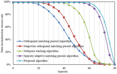
The proposed algorithm was compared with four classic algorithms, namely the orthogonal matching pursuit algorithm, the stagewise orthogonal matching pursuit algorithm, the subspace tracking algorithm, and the sparsity adaptive matching pursuit algorithm. Figures 5 and 6 show the curves of the reconstruction success rate of central heating temperature monitoring data under different sparsities and different numbers of measurement. The upper limit for the number of reconstructions is 1000, and the reconstruction success rate is the number of successful reconstructions divided by 1000.
Figure 5. Curve of the reconstruction success rate under different sparsities
It can be seen from Figure 5 that the data reconstruction success rates of the 5 algorithms, including the algorithm proposed in this paper, decreased as the sparsity increased. As the sparsity changed from small to large, the reconstruction success rate of the proposed algorithm was always higher than those of other algorithms, and it only gradually decreased when the sparsity reached 60.
Figure 6. Curve of the reconstruction success rate under different numbers of measurement
It can be seen from Figure 6 that the data reconstruction success rates of the five algorithms all increased continuously with the increase of the number of measurements. When the number of measurements changed from small to large, the reconstruction success rate of the algorithm proposed in this paper was always higher than those of others, and when the number of measurements reached 60, the rate exceeded 80% while those of other algorithms were all less than 80%. The reconstruction success rates of the orthogonal matching pursuit algorithm, the stagewise orthogonal matching pursuit algorithm, and the subspace tracking algorithm were only about 30%.
Figure 7. Comparison of the reconstruction effects of compressed sensing measurement matrices
Figure 7 shows the simulation results of the reconstructed characteristics of the EMD measurement matrix established in this paper. From Figure 7, it can be seen that the data reconstruction success rates of the reconstruction algorithms based on the stochastic Gaussian matrix and the measurement matrix established in this paper increased as the number of measurements increased. The reconstruction algorithm based on the measurement matrix established in this paper already achieved a certain success rate when the number of measurements was less than 10, while the reconstruction algorithm based on the stochastic Gaussian matrix did not achieve a successful case until the number of measurements reached about 30.
When the number of measurements was small, the measurement matrix established in this paper can obtain a reconstruction success rate of 100%, showing that it has a better overall reconstruction effect.
The following example shows the real-time monitoring of the operating status of the heating stations conducted by the integrated central heating information monitoring system for smart cities under the following three different regulation modes, namely the heating quality regulation mode, the heating flow regulation mode, and the staged integrated heating regulation mode. By collecting the system operating parameters including the outdoor temperature, supply water temperature, return water temperature, heat supplied and flow, this paper summarized the parameters of the heating quality regulation mode, as shown in Table 1.
By collecting the operating parameters of the heat exchange stations in the heating flow regulation mode, and comparing and analyzing the data according to the above method, this paper further summarized the parameters of the heating flow regulation mode, as shown in Table 2.
In the actual central heating system, the design supply water and return water temperatures of the primary pipe network were around 110℃ and 60℃, while those of the secondary pipe network around 80℃ and 50℃. The staged integrated heating regulation mode was adopted for the primary network adopted, and the heating quality regulation mode was adopted for the secondary network. Table 3 shows the calculation results of the operating parameters of the primary and secondary networks.
Before the heating period of the integrated central heating information monitoring system for smart cities proposed in this paper, the heating control system of the 35 heat exchange stations underwent energy-conservation modification and optimization. The total area of the heating monitoring area is 3.2×10⁶m2, and the heating areas of the five core heat exchange stations are 1.94×10⁵m2, 2.31×10⁶m2, 6.01×10⁶m2, 1.94×10⁶m2, and 1.49×10⁶m2. The total heat supplied by the heat source plant during the heating period from 2019 to 2020 was 1.47×10⁶GJ. Based on the standard temperature, Table 4 compares the heat consumptions of the heat source plant and the five core heat exchange stations.
This paper compares the actual energy saved after the heating control system underwent the energy-conservation optimization. Table 5 compares the coal consumption, power consumption, and water consumption after the energy-conservation optimization. It can be seen that, after the energy-conservation optimization, the water, power and coal consumptions have all been reduced to a greater extent. The energy saving effect on electric power is more obvious than those on coal and water. Strengthening the comprehensive monitoring and management of central heating information can effectively reduce different types of energy consumptions, save central heating costs, and improve the utilization efficiency of heating equipment.
Table 1. Parameters of the heating quality regulation mode
|
No. |
1 |
2 |
3 |
4 |
5 |
6 |
7 |
8 |
9 |
10 |
|
Outdoor temperature |
-8 |
-7 |
-6 |
-5 |
-4 |
-3 |
-2 |
-1 |
0 |
1 |
|
Supply water temperature |
86 |
87 |
85 |
84 |
82 |
80 |
79 |
77 |
76 |
75 |
|
Return water temperature |
60 |
58 |
56 |
55 |
54 |
52 |
51 |
49 |
48 |
47 |
|
Heat supplied |
8952 |
8736 |
8571 |
8254 |
8137 |
7952 |
7821 |
7683 |
7534 |
7256 |
|
Flow |
249 |
249 |
249 |
249 |
249 |
249 |
249 |
249 |
249 |
249 |
Table 2. Parameters of the heating flow regulation mode
|
No. |
1 |
2 |
3 |
4 |
5 |
6 |
7 |
8 |
9 |
10 |
|
Outdoor temperature |
-8 |
-7 |
-6 |
-5 |
-4 |
-3 |
-2 |
-1 |
0 |
1 |
|
Return water temperature |
86/62 |
86/62 |
86/62 |
86/62 |
86/62 |
86/62 |
86/62 |
86/62 |
86/62 |
86/62 |
|
Heat flow |
8924 |
8651 |
8427 |
8345 |
8214 |
7823 |
7635 |
7542 |
7354 |
7125 |
|
Heat |
249 |
243 |
235 |
228 |
221 |
215 |
207 |
197 |
192 |
191 |
|
Rotating speed |
1620 |
1530 |
1470 |
1380 |
1350 |
1290 |
1250 |
1160 |
1130 |
1130 |
|
Power of the water pump motor |
27 |
18.5 |
18 |
16 |
12 |
11 |
9 |
8.5 |
7 |
7 |
Table 3. Calculation results of the operating parameters of the primary and secondary pipe networks
|
Load ratio |
|
0.3 |
0.4 |
0.5 |
0.6 |
0.66 |
0.7 |
0.8 |
0.9 |
1.0 |
|
Primary network |
Flow ratio |
0.6 |
0.6 |
0.6 |
0.6 |
0.56 |
0.67 |
0.68 |
0.82 |
1 |
|
Supply water temperature |
68.6 |
82.3 |
96.1 |
110.7 |
122 |
122 |
122 |
122 |
122 |
|
|
Return water temperature |
37.9 |
42.6 |
46.9 |
51.2 |
53.9 |
55.2 |
59.6 |
64.9 |
71 |
|
|
Secondary network |
Flow ratio |
1 |
1 |
1 |
1 |
1 |
1 |
1 |
1 |
1 |
|
Supply water temperature |
43.2 |
49.6 |
56.1 |
62.8 |
66.9 |
68.8 |
74.15 |
79.8 |
86 |
|
|
Return water temperature |
35.9 |
39.7 |
43.8 |
48.2 |
50.2 |
50.8 |
53.9 |
57.8 |
60.5 |
Table 4. Comparison of the heat consumptions of the heat source plant and the 5 core heat exchange stations
|
Description |
Heat source plant |
Heat exchange station 1 |
Heat exchange station 2 |
Heat exchange station 3 |
Heat exchange station 4 |
Heat exchange station 5 |
|
Actual total heat consumption |
138915.25 |
97517.85 |
139551.32 |
285613.78 |
105203.56 |
81956.25 |
|
Heat consumption per unit of area |
0.556 |
0.543 |
0.565 |
0.561 |
0.574 |
0.568 |
|
Converted total heat consumption |
1294531.90 |
87651.25 |
131463.32 |
258433.19 |
98523.25 |
78212.35 |
|
Converted heat consumption per unit of area |
0.505 |
0.473 |
0.485 |
0.492 |
0.457 |
0.513 |
Table 5. Comparison of coal consumption, power consumption and water consumption after energy conservation optimization
|
/ |
Before optimization |
After optimization |
Volume saved |
Saving rate |
|
Annual coal consumption |
92000 |
65700 |
27800 |
35% |
|
Annual power consumption |
12000000 |
5731762.9 |
5572608.2 |
55% |
|
Annual water consumption |
197000 |
160000 |
34000 |
19% |
|
Annual energy consumption cost |
6172.35 |
4154.86 |
1876.74 |
33.6% |
This paper studied the design and implementation of the integrated central heating information monitoring system for smart cities. First, the big data of central heating temperature monitoring in smart cities were reconstructed, the reconstruction principle and the steps to establish the compressed sensing measurement matrix and to reconstruct the central heating temperature monitoring data elaborated, and then the three different central heating regulation modes of the integrated central heating information monitoring system, namely, the heating quality regulation mode, the heating flow regulation mode and the staged integrated heating regulation mode, were introduced. The experimental results show that the reconstruction success rate curve of the central heating temperature monitoring data under different sparsity and different numbers of measurement, which verify that the reconstruction success rate of the algorithm proposed in this paper is always higher than those of other algorithms. The simulation results of the reconstructed characteristics of the established EMD measurement matrix were given in this paper, which show that the measurement matrix established in this paper can obtain a reconstruction success rate of 100% if the measurement number is small. In the instance study, the parameters of the heating quality and flow regulation modes and the calculation results of the operating parameters of the primary and secondary pipe networks were given, and the energy efficiency analysis was performed on the energy-conservation optimization of the system.
[1] Yuan, J., Zhou, Z., Huang, K., Han, Z., Wang, C., Lu, S. (2021). Analysis and evaluation of the operation data for achieving an on-demand heating consumption prediction model of district heating substation. Energy, 214: 118872. https://doi.org/10.1016/j.energy.2020.118872
[2] Wang, C., Nie, P.Y. (2018). How rebound effects of efficiency improvement and price jump of energy influence energy consumption? Journal of Cleaner Production, 202: 497-503. https://doi.org/10.1016/j.jclepro.2018.08.169
[3] Han, H., Wu, S. (2018). Rural residential energy transition and energy consumption intensity in China. Energy Economics, 74: 523-534. https://doi.org/10.1016/j.eneco.2018.04.033
[4] Gao, Z., Cheng, G., Yang, H., Xue, X. (2021). Heating-assisted preparation of ferrotitanium to recover valuable elements of ilmenite and reduce aluminum consumption. JOM, 73(5): 1321-1327. https://doi.org/10.1007/s11837-021-04591-4
[5] Wang, C., Du, Y., Li, H., Wallin, F., Min, G. (2019). New methods for clustering district heating users based on consumption patterns. Applied Energy, 251: 113373. https://doi.org/10.1016/j.apenergy.2019.113373
[6] Wang, R., Lu, S., Li, Q. (2019). Multi-criteria comprehensive study on predictive algorithm of hourly heating energy consumption for residential buildings. Sustainable Cities and Society, 49: 101623. https://doi.org/10.1016/j.scs.2019.101623
[7] Raluy, R.G., Guillén-Lambea, S., Serra, L. M., Guadalfajara, M., Lozano, M.A. (2021). Environmental assessment of central solar heating plants with seasonal storage located in Spain. Journal of Cleaner Production, 314: 128078. https://doi.org/10.1016/j.jclepro.2021.128078
[8] Tyrala, D., Pawlowski, B. (2021). Failure analysis of premature corrosion of HF seam-welded steel pipe in central heating system. Journal of Failure Analysis and Prevention, 21(3): 772-778. https://doi.org/10.1007/s11668-021-01134-6
[9] Hu, J., Wang, K., Zou, X., Shi, B. (2020). Effects of swirl on the heating process of a central gas stream in a tubular flame. Experimental Thermal and Fluid Science, 119: 110209. https://doi.org/10.1016/j.expthermflusci.2020.110209
[10] Behzad, M., Kim, H., Behzad, M., Behambari, H.A. (2019). Improving sustainability performance of heating facilities in a central boiler room by condition-based maintenance. Journal of Cleaner Production, 206: 713-723. https://doi.org/10.1016/j.jclepro.2018.09.221
[11] Topkafa, M., Ayyildiz, H.F. (2017). An implementation of central composite design: Effect of microwave and conventional heating techniques on the triglyceride composition and trans isomer formation in corn oil. International Journal of Food Properties, 20(1): 198-212. https://doi.org/10.1080/10942912.2016.1152481
[12] Yang, X., Svendsen, S. (2018). Ultra-low temperature district heating system with central heat pump and local boosters for low-heat-density area: Analyses on a real case in Denmark. Energy, 159: 243-251. https://doi.org/10.1016/j.energy.2018.06.068
[13] Piana, E.A., Grassi, B., Bianchi, F., Pedrotti, C. (2018). Hydraulic balancing strategies: A case study of radiator-based central heating system. Building Services Engineering Research and Technology, 39(3): 249-262. https://doi.org/10.1177%2F0143624417752830
[14] Comodi, G., Lorenzetti, M., Salvi, D., Arteconi, A. (2017). Criticalities of district heating in Southern Europe: Lesson learned from a CHP-DH in Central Italy. Applied Thermal Engineering, 112: 649-659. https://doi.org/10.1016/j.applthermaleng.2016.09.149
[15] Liu, W. (2021). Energy consumption analysis and comprehensive energy efficiency evaluation of campus central heating system based on heat supply monitoring platform. International Journal of Heat and Technology, 39(3): 746-754. https://doi.org/10.18280/ijht.390308
[16] Schuetz, P., Melillo, A., Businger, F., Durrer, R., Frehner, S., Gwerder, D., Worlitschek, J. (2020). Automated modelling of residential buildings and heating systems based on smart grid monitoring data. Energy and Buildings, 229: 110453. https://doi.org/10.1016/j.enbuild.2020.110453
[17] Parhizkar, T., Aramoun, F., Esbati, S., Saboohi, Y. (2019). Efficient performance monitoring of building central heating system using Bayesian Network method. Journal of Building Engineering, 26: 100835. https://doi.org/10.1016/j.jobe.2019.100835
[18] Burgas, L., Colomer, J., Melndez, J. (2015). Modelling transitions on heating usage in buildings with multivariate statistical monitoring. IEEE EUROCON 2015-International Conference on Computer as a Tool (EUROCON), Salamanca, Spain. https://doi.org/10.1109/EUROCON.2015.7313773
[19] Pippia, T., Lago, J., De Coninck, R., De Schutter, B. (2021). Scenario-based nonlinear model predictive control for building heating systems. Energy and Buildings, 247: 111108. https://doi.org/10.1016/j.enbuild.2021.111108