Jian Yu* | Lili Sui | Yirong Xu | Baoming Chi
© 2021 IIETA. This article is published by IIETA and is licensed under the CC BY 4.0 license (http://creativecommons.org/licenses/by/4.0/).
OPEN ACCESS
In recent decades, the network of seismic subsurface fluid observatories is developing constantly, the observation data of subsurface fluids are enriched accordingly, which provides a favorable condition for the research on the formation, occurrence, and development of earthquakes. In the observation data of subsurface fluids, water level and water temperature changes are very important observation indicators, and their fluctuation sequences are quite complicated. Therefore, this paper employed a non-linear cross-correlation method to study the relationship between the water level and water temperature of Huize Well from 2004 to 2006, and found that there’s a significant cross-correlation between the time series of water level and water temperature; then, this study adopted DCCA (detrended cross-correlation analysis) to calculate the cross-correlation coefficient under different scales and explore the continuous changes of water level and water temperature; at last, this paper used the MF-DCCA (Multifractal-DCCA) method to prove that there’s multifractal cross-correlation between the time series of water level and water temperature. Before the M5.1 earthquake in Huize area, there’s an abnormal increase in the width of the multifractal spectrum of the water level and water temperature drawn with a sliding window of 500-hour, and this is a possible earthquake precursor.
water level, water temperature, MF-DCCA
Subsurface fluids are closely related to the formation, occurrence, and development activities of earthquakes. Under the premise that the confined aquifers of groundwater are in an intact state, the subsurface fluids can flexibly and quickly respond to changes in stress and strain of the earth crust. After the Xingtai earthquake in 1966, China began to establish observation stations to monitor groundwater conditions, after decades of continuous upgrade and perfection, now a subsurface fluid observatory network that can monitor the well water level, temperature, and geochemistry has been constructed. The Earthquake Cases of China recorded that, at the time of the 2004 M8.7 Sumatra earthquake, the water level of 78 wells and the water temperature of 59 wells in China showed co-seismic changes [1]. After researching the co-seismic response mechanism of water level and water temperature of the Tayuan Well in Beijing during multiple earthquakes, scholars Yang et al. [2] believe that in the co-seismic response, the convection and mixing of the water body in the well are the causes of the water temperature drop. Shi et al. [3] studied the co-seismic water level and water temperature changes of the Tangshan Mine Well during 11 earthquakes of magnitude 7.0 or above in 2004, and found that when the well water was vertically oscillated, the disturbed well water triggered a dispersion effect and resulted in changes in the water temperature. During multiple major earthquakes occurred from 2008 to 2013, the water level changes of Jiangsu Well were mostly fluctuations, and the water temperature changes were mostly step changes or trend changes, and the changes of water level and temperature all increased with the increase of the magnitude of the earthquake, and decreased with the increase of the distance from the well to the epicenter [4]. Zhang et al. studied the changes in water level and temperature of Huize Well from 2003 to 2006 and found that there’re obvious relevance, synchronization, and differences between the trend changes of water level and water temperature, and they think such differences are the anomalies before the earthquake [5]. Wang et al. [6] researched the abnormal changes in water level and water temperature and their mechanisms in medium-term, short-term, and short-term stages before the 2014 M4.3 Anhui Shuoshan earthquake. Studies on the fluctuations of water level and water temperature during and before earthquakes play an important role in exploring the formation, occurrence, and development of earthquakes, and such studies can provide important references for pre-earthquake prediction.
Current studies concerning the correlation between water level and water temperature generally use the traditional statistical methods, such as the Pearson's correlation coefficient method, and the linear regression method, etc. However, since the changes in the water level and temperature of monitoring wells are complicated and the time series are unstable, some non-linear correlation methods might be more suitable. At present, the fractal method has been effectively applied to the searching of abnormal soil radon content or electromagnetic anomalies before earthquakes [7-16]. Kar et al. [17] proposed to apply MF-DCCA to study the relationship between soil radon content and temperature anomaly, and they found that temperature anomaly and soil radon content exhibited varying degrees of complexity and multifractal cross-correlation. This paper attempts to use MF-DCCA to explore the non-linear correlation between the water level and water temperature of seismic monitoring wells, namely the multifractal cross-correlation.
In our study, water level and water temperature data of Huize Well from 2004 to 2006 were selected for analysis; at first, the cross-correlation test was carried out to verify that there’s a cross-correlation between water level and water temperature; then, DCCA was used to obtain the cross-correlation coefficient of water level and water temperature under different scales; after that, the MF-DCCA method was adopted to verify the multifractal cross-correlation between the time series of water level and water temperature; at last, this paper used MF-DCCA to figure out the changes in multifractal cross-correlation between water level and water temperature in the sliding window.
The data used in this study are the water level and water temperature data of Huize Well from January 1, 2004 to December 31, 2006, the well is located in Huize County, Qujing City, Yunnan Province, China; its geographical coordinates are 26.52°N, 103.15°E; the altitude of the well head is 2005 meters above sea level, and the well is located at the margin of the Nagu Lake Basin, 8 km east of the Xiaojiang Fault. The landforms of this area are mainly mountainous and basins. The groundwater is confined fissure water, and the lithology of the aquifer is weathered basalt, gravel, broken stone, and sand gravel. The well depth is 103.15m; the burial depth of the water level is about 30.00 m; the depth of the casing pipe is 87.80m, of which 34.06-87.80m is the filter pipe, and the observation section is 34.06-103.15m. The well water level data is from the China Earthquake Networks Center (CENC) and the website of seismic subsurface fluids. The instruments used for monitoring the water level and water temperature of the Huize Well are respectively the Model LN-3 digital water level meter and the Model SZW-1A digital thermometer. Data of the sampling rate are all in minutes. In this paper, the minute data of water level and temperature of the Huize Well were converted into data in hours, and the missing data were filled in using a cubic polynomial fitting method.
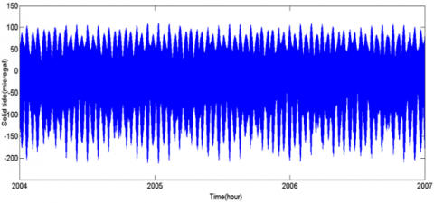
As shown in Figure 1, during the observation years, the water level and temperature of Huize Well showed a gradual decline, and was not affected by rainfall. The water level decline speed was 0.3 m per year, the effect of air pressure was not obvious, and there’s an earth tide effect with no annual change; the water temperature decline speed was 0.0045℃ each year, and there’s no annual change. Huize Well is well enclosed, its sensitivity is high, and its water level and temperature anomalies are significantly related to seismic activities. Table 1 lists the information of 4 earthquakes, during the first three earthquakes, the well water level and temperature showed obvious changes after the earthquakes, while the respond for the fourth earthquake was not obvious. When the seismic wave generated by the earthquake reached the monitoring well, it will cause deformation to the aquifer of the well, change the pressure in the pores and fissures, and result in changes in the water level and temperature. When the pressure in pores and fissures increases, the groundwater in the aquifer flows into the monitoring well, the well water moves upward under the pressure, so the water level rises; otherwise, the water level drops. At this time, if the water temperature has a positive gradient, then the water temperature will rise; if the water temperature has a negative gradient, the water level will drop [18].
Figure 1. Time series of water level and water temperature of Huize Well from 2004 to 2006
Table 1. Information of four major earthquakes in Yunnan from 2004 to 2006
|
No. |
Date |
Place |
Magnitude |
Longitude |
Latitude |
Distance from the well to the epicenter (km) |
|
1 |
2004.08.10 |
Ludian, Yunan |
5.6 |
103.6 |
27.2 |
87.81 |
|
2 |
2005.08.05 |
Huize, Yunnan |
5.3 |
103.1 |
26.6 |
10.19 |
|
3 |
2006.07.22 |
Yanjin, Yunnan |
5.1 |
104.2 |
28 |
194.56 |
|
4 |
2006.08.25 |
Yanjin, Yunnan |
5.1 |
104.2 |
28 |
194.56 |
3.1 Cross-correlation test
The cross-correlation statistic test can examine whether two groups of time series $\left\{x_{t}, \mathrm{t}=1,2, \cdots, \mathrm{N}\right\}$ and $\left\{y_{t}, \mathrm{t}=1,2, \cdots, \mathrm{N}\right\}$ have long-range cross-correlation [19], wherein the cross-correlation function Ci and the cross-correlation statistic $Q_{c c}(m)$ are defined as follows:
$C_{i}=\frac{\sum_{k=i+1}^{N} \quad x_{k} y_{k-i}}{\sqrt{\sum_{k=1}^{N} \quad x_{k}^{2} \sum_{k=1}^{N} \quad y_{k}^{2}}}$, (1)
$Q_{c c}(m)=N^{2} \sum_{i=1}^{m} \frac{c_{i}^{2}}{N-i}$ (2)
The statistic $Q_{c c}(m)$ approximately obeys the $\chi^{2}(m)$ distribution with m degrees of freedom. Within the value range of freedom degree m, if statistic is consistent with the critical value $\chi^{2}(m)$ at the significance level of 5%, then there is no cross-correlation between the two time series; if statistic $Q_{c c}(m)$ is greater than critical value $\chi^{2}(m)$ at the significance level of 5%, then there is a cross-correlation between the two time series.
3.2 DCCA
The DCCA (detrended cross-correlation analysis) method [20] has extended the traditional correlation analysis methods which can only process stationary time series, DCCA can process non-stationary time series, and its specific steps are:
(1) Assume there’re two time series $\left\{x_{t}, \mathrm{t}=1,2, \cdots, \mathrm{N}\right\}$ and $\left\{y_{t}, \mathrm{t}=1,2, \cdots, \mathrm{N}\right\}$, calculate their sums as:
$\left\{ \begin{matrix} {{R}_{k}}=\sum\limits_{i=1}^{k}{{{x}_{i}},k=1,\cdots ,N} \\ {{{{R}'}}_{k}}=\sum\limits_{i=1}^{k}{{{y}_{i}},k=1,\cdots ,N} \\ \end{matrix} \right.$ (3)
(2) Divide the two cumulative time series into N-n overlapping time slots, and each time slot contains n+1 values. The time slot starts at i and ends at i+n.
(3) In each time slot, the two cumulative time series are respectively fitted using the least squares method to obtain trends of local time slots $\widetilde{R_{k, l}}$ and $\widetilde{R_{k, l}^{\prime}}$.
(4) In each time slot, get the residuals of two original cumulative time series and their respective local fitted time series trends, and calculate the covariance of their residuals:
$f_{DCCA}^{2}(n,i)=\frac{1}{n-1}\sum\limits_{k=i}^{i+n}{({{R}_{k}}-\widetilde{{{R}_{k,i}}})}({{{R}'}_{k}}-\widetilde{{{{{R}'}}_{k,i}}})$ (4)
(5) Calculate the covariance of the entire time series on different time scales:
$F_{DCCA}^{2}=\frac{1}{N\text{-}n}\sum\limits_{i=1}^{N-n}{f_{DCCA}^{2}}(n,i)$ (5)
Calculate Formula (5) repeatedly on each time scale, then we can get:
${{F}_{DCCA}}(n)\sim {{n}^{\lambda }}$ (6)
$\lambda$ is the scale parameter, it can reflect the cross-correlation of two time series. When $0<\lambda<0.5$, it means that the two time series have long-range negative correlation; when $0.5<\lambda<1$, it means that the two time series have long-range positive correlation. When $R_{k}=R_{k}^{\prime}$, the detrended covariance $F_{D C C A}^{2}(n)$ becomes the detrended variance $F_{D F A}^{2}(n)$. Since the DCCA scale parameter $\lambda$ cannot strictly quantify the correlation between the two time series, so the detrended variance DFA was added to obtain the detrended correlation coefficient $\rho_{D C C A}$, which is:
$\rho_{D C C A}=\frac{F_{D C C A}^{2}\quad(n)}{F_{X D F A}\quad(n) F_{Y D F A}\quad(n)}$ (7)
where, $F_{X D F A}(n)$ and $F_{Y D F A}(n)$ are the DFA scale parameters of the two time series $\left\{x_{t}, \mathrm{t}=1,2, \cdots, \mathrm{N}\right\}$ and $\left\{y_{t}, \mathrm{t}=1,2, \cdots, \mathrm{N}\right\}$. The DCCA method is different from the traditional Pearson correlation coefficient method, Pearson correlation coefficient is applicable to stationary time series, while the DCCA has extended to non-stationary time series. The traditional Pearson correlation coefficient has a unique value, while DCCA obtains different correlation coefficient values for different time scales.
3.3 MF-DCCA
Zhou [21] combined multifractal method with DCCA and proposed the MF-DCCA method, namely multifractal detrended cross-correlation analysis, it is also a research method for non-stationary time series.
The specific steps are as follows:
(1) For two given time series $\left\{x_{t}, \mathrm{t}=1,2, \cdots, \mathrm{N}\right\}$ and $\left\{y_{t}, \mathrm{t}=1,2, \cdots, \mathrm{N}\right\}$, N is the length of the time series, calculate the cumulative deviation sums of their mean values, and generate new series $X(i)$ and $Y(i)$:
$X(i)=\sum_{t=1}^{i}(x(t)-\bar{x}) \quad, Y(i)=\sum_{t=1}^{i}(y(t)-\bar{y})$ (8)
where, $\bar{x}$ and $\bar{y}$ are the mean values of the two time series.
(2) Divide the two time series $X(i)$ and $Y(i)$ into $N_{S}$ sub-intervals. The length of each interval is s, and there’s no overlap between each interval, wherein $N_{s}=\operatorname{int}(N / S)$. Since for most time series, the length N might not be divided exactly by s, that is, there might be residual data that is less than length s. In order to make full use of the data, the first and last data of the two series $X(i)$ and $Y(i)$ are reversed, and the series are re-divided for more than once, then $2 N_{s}$ subintervals are obtained:
(3) In each sub-interval, the time series are fitted by the least squares method to generate two fitted series $x_{\lambda}$ and $y_{\lambda}$, which are then detrended to obtain the covariance function as follows:
when $\lambda=1,2, \cdots, N_{s}$,
$\begin{align} & {{F}^{2}}(s,\lambda )=\frac{1}{s}\sum\limits_{i=1}^{s}{(X((\lambda -1)s+i)-{{x}_{\lambda }}(i))} \\ & \times (Y((\lambda -1)s+i)-{{y}_{\lambda }}(i)) \\ \end{align}$ (9)
when $\lambda=N_{s}+1, \cdots, 2 N_{s}$,
$\begin{align} & {{F}^{2}}(s,\lambda )=\frac{1}{s}\sum\limits_{i=1}^{s}{(x(N-(\lambda -{{N}_{s}})s+i)-{{x}_{\lambda }}(i))} \\ & \times (Y(N-(\lambda -{{N}_{s}})s+i)-{{y}_{\lambda }}(i)) \\ \end{align}$ (10)
(4) Take the mean value of the covariance in each sub-interval, and calculate the q-order fluctuation function:
${{F}_{q}}(s)={{(\frac{1}{2{{N}_{s}}}\sum\limits_{\lambda =1}^{2{{N}_{s}}}{({{F}^{2}}{{(s,\lambda )}^{\frac{q}{2}}})})}^{\frac{1}{q}}}$ (11)
when $q=0$,
${{F}_{0}}(s)=\exp (\frac{1}{4{{N}_{s}}}\sum\limits_{\lambda }^{2{{N}_{s}}}{(\ln {{F}^{2}}(s,\lambda ))})$ (12)
(5) The power-law relationship between the fluctuation function $F_{q}(s)$ and time interval s under different scales s is:
$F_{q}(s) \sim s^{H(q)}$, namely: $\log F_{q}(s)=H(q) \log (s)+\log C$
where, $H(q)$ is the generalized Hurst exponent.
(6) The multifractal scale index is $\tau(q)$, and its relationship with the generalized Hurst exponent is:
$\tau (q)=qH(q)-1$
If $\tau(q)$ and $q$ have a non-linear relationship, then the two time series have multifractal characteristics, otherwise they are single fractal.
(7) Through Legendre transformation, the multifractal spectrum is obtained as:
$\alpha (q)=H(q)+{H}'(q)$
$f(\alpha )=q(\alpha (q)-H(q))+1$
where, $\alpha$ is the singularity index of the time series, $f(\alpha)$ is the multifractal spectrum, wherein the width of the multifractal spectrum is $\Delta \alpha=\alpha \min _{\max }$. The greater the width of the multifractal spectrum, the stronger the multifractals of the cross-correlation of the two time series, and the more obvious the long-range cross-correlation; otherwise, the weaker the multifractals and the long-range cross-correlation. $\Delta f=f\left(\alpha_{\min }\right)-f\left(\alpha_{\max }\right)$ is the difference of the multifractal spectra. When $\Delta f>0$, the multifractal spectrum shows left skew, it means that it is of higher probability that the two time series are of greater values, and they have a rising trend; when $\Delta f<0$, the multifractal spectrum shows right skew, it means that that it is of higher probability that the two time series are of smaller values, and they have a decline trend.
4.1 Cross-correlation test
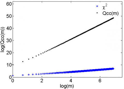
First, the water level and water temperature data (in hour) of the Huize Well from January 1, 2004 to December 31, 2006 were supposed to be two sequences $\left\{x_{i}, \mathrm{i}=1,2, \cdots, \mathrm{N}\right\}$ and $\left\{y_{i}, \mathrm{i}=1,2, \cdots, \mathrm{N}\right\}$, respectively, and $N=26303$. Then, the cross-correlation test was performed on the time series fluctuations of the water level and temperature of Huize Well, as shown in Figure 2, the black dots are the cross statistic $Q_{c c}(m)$, wherein the value of m (degree of freedom) was $1 \sim 1000$; the blue dots are the critical values of $\chi^{2}(m)$ under a significance level of 5%; Within the value range of the degree of freedom, the cross-correlation statistics were larger than the critical values of the corresponding chi-square distribution, that is, the time series of the water level and the water temperature of the Huize Well have a significant cross-correlation.
Figure 2. Cross-correlation test on the time series of water level and water temperature of Huize Well from 2004 to 2006
4.2 Detrended cross-correlation coefficient $\rho D C C A$
The value range of the detrended cross-correlation coefficient $\rho D C C A$ is between $[-1,1]$. If $\rho_{D C C A}$=0, there is no cross-correlation between the two; if $\rho_{D C C A}=-1$, then the two time series have a complete negative persistent correlation; if $\rho_{D C C A}=1$, then the two time series have a complete positive persistent correlation. Based on different scales, the polynomial adopted in the least square fitting took an order of 2, and the different cross-correlation coefficients were calculated. As can be seen from Table 2 that the time series of the water level and water temperature of Huize Well showed a cross-correlation under all scales, but the positive and negative persistence under different scales were different, indicating that the correlation of water level and water temperature of Huize Well was unstable and the changes were complicated, therefore, the MF-DCCA was adopted to further study the fluctuation relationship between the water level and water temperature of Huize Well.
Table 2. Values of the cross-correlation coefficient under different scales
|
Scale |
2 |
4 |
16 |
32 |
64 |
128 |
256 |
512 |
|
Cross-correlation coefficient |
0.0691 |
0.0027 |
-0.5811 |
-0.1429 |
-0.0671 |
0.0840 |
0.0265 |
-0.0119 |
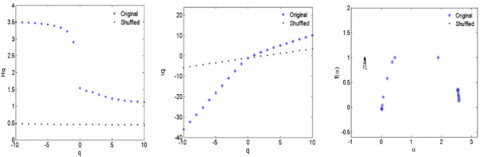
Figure 3. Multifractal results of the overall data of Huize Well from 2004 to 2006
4.3 MF-DCCA
4.3.1 Overall data analysis
The water level and water temperature time series of Huize Well from January 1, 2004 to December 31, 2006 were subject to MF-DCCA to estimate their non-linear cross-correlation and multifractal features, as shown in Figure 3, the Original represents the results of the multifractal features of the original sequence, and the Shuffled represents the results of the random rearrangement of the sequence. It can be seen from Figure 3(a) that, the generalized Hurst decreases with the increase of q, when $q=2$, there is $H(2)>0.5$, and the randomly re-arranged sequence $H(2) \approx 0.5$, indicating that the original water level and water temperature time series had a long-range correlation; as can be seen from Figure 3(b), the relationship between the scale of the multifractal spectrum $\tau(q)$ and q was not linear, indicating that the correlation between water level and water temperature had multifractal features; while the scale of the multifractal spectrum of the randomly re-arranged sequence $\tau(q)$ and q had a linear correlation, that is, it was a single fractal. Moreover, as can be seen from Figure 3(c), the width of the multifractal spectrum of the original sequence $\Delta \alpha=2.5712$ was greater than the width of the multifractal spectrum of the randomly re-arranged sequence $\Delta \alpha=0.0788$, and the wider the multifractal spectrum, the stronger the multifractal features, thus, it can be concluded that the long-range cross-correlation of the original water level and water temperature time series was stronger than that of the re-arranged series, and the complexity of the original water level and water temperature fluctuations was higher.
4.3.2 Sliding window analysis
The multifractal cross-correlation of the water level and water temperature time series of Huize Well was also subject to sliding window analysis to figure out its variation features over time, then the multifractal cross-correlation of the detrended high-frequency data of the water level and water temperature of Huize Well could be extracted, and the $Hurst$ exponent, the width of the multifractal spectrum, and the difference of the multifractal spectra could be calculated. In many studies, the width of the multifractal spectrum can reflect the fluctuation characteristics of the time series. The length of the sliding window is very important for studying the correlation; if the sliding window is too long, a lot of local information will be lost; if the sliding window is too short, local fluctuations may be too violent and they may affect the observation of the dynamic trends. In this study, 500h was chosen as the length of the sliding window, starting from the first observation data, the MF-DCCA method was adopted to calculate the Hurst exponent and the width of the multifractal spectrum, then, with 500h as the length, the window slid backward until the remaining time was less than 500h. Figure 4 shows that, with 500h as the sliding window, the water level and water temperature time series of the Huize Well showed long-range correlation.
Figure 4. Hurst exponent between water level and water temperature calculated by MF-DCCA in 500h sliding window
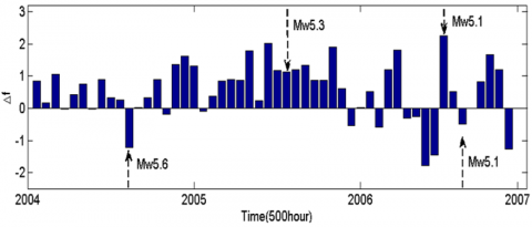
The width of the multifractal spectrum is shown in Figure 5. There’s an interesting discovery with the figure, before the occurrence of the M5.3 Huize earthquake, the width of the multifractal spectrum of the well water level and water temperature increased abnormally, and remained at a high value level for quite a while after the earthquake, and this indicated that the multifractal feature of the cross-correlation between the water level and water temperature fluctuations before the earthquake had been enhanced; as can be seen from Figure 5, within a long period of time before the earthquake, Δf>0, indicating that under the interaction of water level and water temperature, the probability of fluctuation increment was higher, and it showed an increasing trend afterwards. It is believed that this phenomenon of the enlarged multifractal spectrum of the water level and water temperature time series before the earthquake may be the precursor anomalies of the earthquake, which might be caused by factors such as air pressure or earth tide.
For the M5.3 Ludian earthquake and the twice M5.1 Yanjin earthquakes, the interactive relationship between the groundwater level and temperature was quite different from that of the Huize earthquake, before and after the three earthquakes, their multifractal spectra showed no high value, and the width of the multifractal spectra of the three earthquakes was 0.3212, 1.0237, and 0.3719, respectively, that is, the width value of the multifractal spectrum of the temporary water level fluctuations caused by seismic waves was relatively small. From the perspective of the difference of the multifractal spectra, the three earthquakes were studied together and it’s found that among the three, only in the M5.1 Yanjin earthquake occurred on July 2006, there’s Δf>0; while in the other two earthquakes, Δf>0; moreover, the width of the multifractal spectrum of the Yanjin earthquake was wider than that of the other two earthquakes, indicating that the water level and temperature fluctuations in the Yanjin earthquake were more complicated than those of the other two. The causes might be that, there’s no abnormal fluctuation in the well water level and temperature before the earthquakes, and the fluctuations of water level and temperature had only occurred under the action of the seismic waves during the earthquakes.
Figure 5. Width and difference of water level and temperature multifractal spectra in the 500-hour sliding window
Since the high-frequency information of well water level and temperature may contain abnormal information of the earthquakes, and the water level anomalies might be caused by non-tectonic factors, therefore, whether other factors would cause the width of the well water level and temperature multifractal spectrum before the Huize earthquake to increase should be considered. At first, by looking up the changes of the air pressure coefficient, whether the anomaly of the multifractal spectrum width before the Huize earthquake was caused by air pressure could be determined. Based on the air pressure data (in days) from 2004 to 2006, a one-variable linear regression model with a time window of 2 months describing the relationship between air pressure and the water level of Huize well was established to calculate the air pressure coefficient in the response time window.
Table 3. Air pressure coefficient of Huize well
|
Start and end date |
Air pressure coefficient |
Correlation coefficient R |
|
2004/01/01-2004/02/29 |
1.9951 |
0.2624 |
|
2004/03/01-2004/04/30 |
2.1883 |
0.5911 |
|
2004/05/01-2004/06/30 |
3.5701 |
0.4415 |
|
2004/07/01-2004/08/31 |
3.7171 |
0.4319 |
|
2004/09/01-2004/10/31 |
2.6353 |
0.4763 |
|
2004/11/01-2004/12/31 |
3.3889 |
0.7404 |
|
2005/01/01-2005/02/28 |
2.3179 |
0.5250 |
|
2005/03/01-2005/04/30 |
3.0521 |
0.5308 |
|
2005/05/01-2005/06/30 |
2.8560 |
0.4394 |
|
2006/03/01-2006/04/30 |
1.5594 |
0.3027 |
|
2006/05/01-2005/06/30 |
3.9543 |
0.7721 |
The linear regression models that past the significance test in different time windows, namely in those there’s a regression relationship between the air pressure change and the water level change, are shown in the Table 3. In terms of the air pressure coefficient, before the Huize earthquake, there’s no obvious anomaly in the air pressure coefficient, and its value was between 2.3179 and 3.0521, indicating that the high-value anomaly of the multifractal spectrum width before the Huize earthquake had nothing to do with air pressure; in addition, the correlation between the general atmospheric pressure change and the water level change was poor, only the correlation coefficients of 2004/11/01-2004/12/31 and 2006/05/01-2005/06/30 time intervals were above 0.7, therefore, the impact of air pressure on the water level was average.
Figure 6. Data of theoretical of earth tide (in hours) of Huize well from 2004/01/01 to 2006/12/31
In order to determine the relationship between the change of earth tide and the change of water level, the data of the theoretical value of earth tide (in hours) from 2004/01/01 to 2006/12/31 were generated as shown in the following figure 6, again, 2 months were taken as a time window, within which, a one-variable linear regression model with earth tide change as the independent variable and the water level change as the dependent variable was established. However, within 18 time windows, the linear model failed to pass the significance test, indicating that the impact of earth tide on water level was not significant.
The rainy season in Huize area is from May to August (Figure 7). Observation of the water temperature of Huize well shows that the well water temperature has a long-term downward trend, which is a normal dynamic change of the water temperature, and it isn’t affected by the rainfall. The pressure well is considered to be well sealed, that is, the situation that the rainfall would cause high-value anomaly to the width of the multifractal spectrum before Huize earthquake has been excluded.
Figure 7. Data of rainfall (in days) from 2004/01/01 to 2006/12/31
As a result, possible causes of the anomaly in the width of the multifractal spectrum, such as air pressure, earth tide, and rainfall had all be excluded, therefore, this paper believes that the possible reason for such situation might be that, when the mechanical processes generated by the earthquake spread to the aquifer rock mass in the shallow crust, due to the existence of voids (such as pores, cracks, and caves) developed in the rock mass, even a weak mechanical force can cause certain deformation to the voids, or cause some weak parts to generate local cracks, and such deformation and cracks will certainly lead to changes in the pore pressure of the aquifer, thereby affecting the changes in the water flow inside the aquifer system [22-25]. Since the airtight monitoring wells can sensitively respond to small changes in water level and water temperature, and the changes in the interactive relationship of the fluctuations of well water level and temperature are the critical phenomenon of the groundwater level and temperature before earthquakes, the MF-DCCA method can well capture such fluctuation changes. Before and after the M5.3 Huize earthquake, obvious changes in the width of the multifractal spectrum could be observed, and we believe that this might be the precursor of the Huize earthquake. However, this method needs to be further verified by the changes of water level and temperature of more monitoring wells before the earthquakes.
This paper researched the non-linear correlation between the water level and water temperature time series of Huize well during the three years from the beginning of 2004 to the end of 2006, and obtained following conclusions:
(1) The analysis of the cross-correlation test results showed that, the test value of the cross-correlation statistic Qcc(m) of the well water level and water temperature time series was greater than the critical value of $\chi^{2}(m)$, indicating that the water level and water temperature of Huize Well had significant cross-correlation.
(2) Using the DCCA method, it’s calculated that under different scales, the positive and negative features of the detrended correlation coefficient were not stable, indicating that the fluctuation of water level and water temperature was complicated, and this was related to the effect of earthquakes on the well water level and temperature.
(3) The MF-DCCA method was used to analyze the time series of water level and temperature of Huize well from 2004 to 2006, and it’s found that there’s a multi-fractal cross-correlation between the two, and such correlation was long-range and continuous; the width of the multi-fractal spectrum was large, and the re-arranged sequences had single fractal feature. Then, with 500-hour as the sliding window, the window slid backward from January 1, 2004, the MF-DCCA method was applied again, and it’s obtained that within each sliding window, the water level and water temperature had long-range multi-fractal cross-correlation.
(4) This paper studied four earthquakes that occurred in Yunnan Province from 2004 to 2006, and found that before the M5.3 Huize earthquake, the width of the multifractal spectrum increased abnormally, indicating that the multifractal cross-correlation of water level and water temperature had been enhanced; after excluding factors such as air pressure, earth tide, and rainfall, we believe that such anomaly might be the precursor of the Huize earthquake, and the abnormal increase in the width of the multifractal spectrum is a self-organized critical phenomenon before the earthquakes.
(5) The width of the multifractal spectra of the M5.6 Ludian earthquake and the twice M5.1 Yanjin earthquakes was relatively small, indicating that the co-seismic seismic waves had a low impact on the multifractal cross-correlation of water level and water temperature.
[1] Liu, Y.W. (2006). Review of the research progress on the seismological science of underground fluid in China during last 40 years. Earthquake Research in China, 22(3): 222-235. https://doi.org/10.3969/j.issn.0253-4975.2006.07.003
[2] Yang, Z.Z., Deng, Z.H., Tao, J.L., Gu, Y.Z., Wang, Z.M., Liu, C.L. (2007). Coseismic effects of water temperature based on digital observation from Tayuan well, Beijing. Acta Seismologica Sinica, 20(2): 212-223. https://doi.org/10.3321/j.issn:0253-3782.2007.02.010
[3] Shi, Y.L., Cao, J.L., Ma, L., Yin, B.J. (2007). Tele-seismic coseismic well temperature changes and their interpretation. Acta Seismologica Sinica, 20(3): 280-289. https://doi.org/10.3321/ j.issn:0253-3782.2007.03.005
[4] Miao, A.L., Zhang, Y., Ye, B.W., Shen, H.H. (2014). Feature and mechanism of co-seismic responses of Jiangsu groundwater level and temperature to several strong earthquakes. Earthquake, 34(4): 78-87. https://doi.org/10.3969/j.issn.1000-3274.2014.04.009
[5] Zhang, L., Zhao, H.S., Liu, Y.W., Fu, H. (2009). Correlation between water level and water temperature in Huize well in Yunnan: Significance of earthquake prediction. Journal of Seismological Research, 32(3): 228-230. https://doi.org/10.3969/j.issn.1000-0666.2009.03.002
[6] Wang, J., Huang, X.L., Liu, C.J., Li, J.H., He, K., Zheng, H.G., Wang, X.Y., Yang, Y.Y. (2020). Analysis of Typical Anomalies Observed from Underground Fluid before 2014 Huoshan Ms4.3 Earthquake. Earthquake Research in China, 36(1): 67-79. https://doi.org/doi:10.3969/j.issn.1001-4683.2020.01.007
[7] Ghosh, D., Deb, A., Dutta, S., Sengupta, R., Samanta, S. (2012). Multifractality of radon concentration fluctuation in earthquake related signal. Fractals, 20(1): 33-39. https://doi.org/10.1142 /S0218348X12 50003X
[8] Barman, C., Chaudhuri, H., Ghose, D., Deb, A., Sinha, B. (2014). Multifractal detrended fluctuation analysis of seismic induced radon-222 time series. Journal of Earthquake Science and Engineering, 1: 59-79.
[9] Barman, C., Chaudhuri, H., Deb, A., Ghose, D., Sinha, B. (2015). The essence of multifractal detrended fluctuation technique to explore the dynamics of soil radon precursor for earthquakes. Natural Hazards, 78(2): 855-877. https://doi.org/10.1007/s11069-015-1747-1
[10] Telesca, L., Balasco, M., Colangelo, G., Lapenna, V., Macchiato, M. (2004). Investigating the multifractal properties of geoelectrical signals measured in southern Italy. Physics and Chemistry of the Earth, Parts A/B/C, 29(4-9): 295-303. https://doi.org/10.1016/j.pce.2003.09.015
[11] Telesca, L., Lapenna, V., Macchiato, M. (2005). Multifractal fluctuations in earthquake-related geoelectrical signals. New Journal of Physics, 7(1): 214. https://doi.org/10.1088/1367-2630/7/1/214
[12] Aggarwal, S.K., Lovallo, M., Khan, P.K., Rastogi, B.K., Telesca, L. (2015). Multifractal detrended fluctuation analysis of magnitude series of seismicity of Kachchh region, Western India. Physica A: Statistical Mechanics and its Applications, 426: 56-62. https://doi.org/10.1016/j.physa.2015.01.049
[13] Telesca, L., Lovallo, M., Molist, J.M., Moreno, C.L., Meléndez, R.A. (2015). Multifractal investigation of continuous seismic signal recorded at El Hierro volcano (Canary Islands) during the 2011–2012 pre-and eruptive phases. Tectonophysics, 642: 71-77. https://doi.org/10.1016/j.tecto.2014.12.019
[14] Fan, X., Lin, M. (2017). Multiscale multifractal detrended fluctuation analysis of earthquake magnitude series of Southern California. Physica A: Statistical Mechanics and Its Applications, 479: 225-235. https://doi.org/10.1016/ j.physa. 2017.03.003
[15] Sarlis, N.V., Skordas, E.S., Mintzelas, A., Papadopoulou, K.A. (2018). Micro-scale, mid-scale, and macro-scale in global seismicity identified by empirical mode decomposition and their multifractal characteristics. Scientific Reports, 8(1): 1-15. https://doi.org/10.1038/s41598-018-27567-y
[16] Telesca, L., Lapenna, V. (2006). Measuring multifractality in seismic sequences. Tectonophysics, 423(1-4): 115-123. https://doi.org/10.1016/j.tecto.2006.03.023
[17] Kar, A., Chatterjee, S., Ghosh, D. (2019). Multifractal detrended cross correlation analysis of land-surface temperature anomalies and Soil radon concentration. Physica A: Statistical Mechanics and its Applications, 521: 236-247. https://doi.org/10.1016/j.physa.2019.01.056
[18] Zhang, B., Liu, Y.W., Gao, X.Q., Yang, X.H., Ren, H.W., Li, Y.W. (2015). Correlation analysis on co-seismic response between well water level and temperature caused by the Nepal M_S8.1 earthquake. Acta Seismologica Sinica, 37(4): 533-540+711. https://doi.org/10.11939/jass.2015.04.001
[19] Podobnik, B., Grosse, I., Horvatić, D., Ilic, S., Ivanov, P.C., Stanley, H.E. (2009). Quantifying cross-correlations using local and global detrending approaches. The European Physical Journal B, 71(2): 243-250. https://doi.org/10.1140/epjb/e2009-00310-5
[20] Podobnik, B., Stanley, H.E. (2008). Detrended cross-correlation analysis: A new method for analyzing two nonstationary time series. Physical Review Letters, 100(8): 084102. https://doi.org/10.1103/PhysRevLett.100.084102
[21] Zhou, W.X. (2008). Multifractal detrended cross-correlation analysis for two nonstationary signals. Physical Review E Statistical Nonlinear & Soft Matter Physics, 77(6): 066211. https://doi.org/10.1103/PhysRevE.77.066211
[22] Che, Y.T., He, A.H., Yu, J.Z. (2014). Mechanisms of water-heat dynamics and earth-heat dynamics of well water temperature micro-behavior. Acta Seismologica Sinica (in Chinese), 36(1): 106-117. https://doi.org/10.3969/j.issn.0253-3782.2014.01.009
[23] Che, Y.T., Liu, C.L., Yu, J.Z. (2008). Micro-behavior of well water temperature and its mechanism. Earthquake, 28(4): 20-28. https://doi.org/10.3969/j.issn.1000-3274.2008.04.003
[24] Yu, J.Z., Che, Y.T. Liu, W.Z. (1997). Preliminary study on hydrodynamic mechanism of microbehavior of water temperature in well. Earthquake, 17(4): 389-396.
[25] Yang, Q.Y., Zhang, Y., Fu, L.Y., Zhang, W., Hu, J.H., Huang, F.Q., Cao, C.H. (2020). Coupling mechanism of stress variation and groundwater (water level, water temperature, hydrochemistry, soil gas, etc.) and its application in earthquake precursors research in Sichuan and Yunnan regions. Progress in Geophysics, 35(6): 2124-2133. https://doi.org/10.6038/pg2020DD0404