Prosper Gopdjim Noumo* | Donatien Njomo | Kevin Zepang Nana | Leonard Ribot Chuisseu Nguewo
© 2021 IIETA. This article is published by IIETA and is licensed under the CC BY 4.0 license (http://creativecommons.org/licenses/by/4.0/).
OPEN ACCESS
This paper considered an existing subsea pipeline transporting an oil and gas flow, and proposed to find the best thermal insulating material and the required thickness of insulation necessary to meet an output temperature of 40℃ and a pressure of 2.4MPa so as to avoid flow assurance issues. MATLAB and PIPESIM software were employed to run the simulations of the temperature and pressure profiles along the considered pipeline. Data used for the simulations were obtained from open literature. Results obtained from our simulations in MATLAB are validated using PIPESIM software, measured values and prediction model from literature. The temperature model was then used to thermally design an insulation thickness for the 50 km long pipeline using three insulating materials which are: black aerogel, polyurethane and calcium silicate. Results from the analysis showed that the black Aerogel material with a critical thickness of 10.16 cm is most effective to satisfy the criterion design. The effect of the selected insulating material was also investigated on the phase envelop. Results shows that for proper insulation thickness the flowing fluid temperature can be maintained at a temperature above which no flow assurance issues can be observed.
thermal insulation, two-phase flow, heat transfer, numerical simulation, temperature profile, pressure profile
In deepwater oil production project, where wells are located far from platforms, offshore fluids generally consisting of oil gas and water are often transported over long distances in subsea pipelines [1]. During the transportation, the multiphase fluids is cooled on its way to the surface production due to heat transfer, through the pipelines walls, with the surrounding seawater [1]. If the production flow-line is not properly and sufficiently insulated against heat losses to the external surrounding, temperature of the flowing fluids inside the subsea pipeline will drop and this may lead to some flow assurance issues such as the precipitation of asphaltenes and/or paraffin wax and the formation of hydrates [2]. For example, it is shown by Ahmed [3] that at temperature around 288, 15°k, wax will start to form inside the pipeline and at temperature below 313, 15°k, combine with high-pressure gas hydrates will occur. As results of these issues, pipe effective flow area may reduce and if serious, blockage may occur [4]. In subsea area, the interaction between the cold surrounding water and the warm flowing fluids inside pipeline is a major cause of temperature drop, which is responsible of some flow assurance issues such as wax deposition, and risk of hydrates formation. Therefore, temperature drops must be prevented in oil and gas production in order to minimize flow assurance issues. This can be achieved by choosing a proper insulation material with an appropriate thickness for the pipeline.
Insulation of pipeline is becoming more and more increasingly important in any subsea project because of the increase in energy saving that it can provides. Optimum insulation thickness need then to be calculated for an appropriate selection of the insulating material with respect to a proper thickness. In recent years, many researches have been carried out on this topic in the open literature showing the interest of scientific for the pipeline thermal design. For examples: Nurfarah and William [5] carried out a study on the optimum thermal insulation design for subsea pipeline. One of theirs objectives was to establish a workflow procedure in selecting thermal insulation materials, thickness and number of layers required for protective coating. The pipeline length considered was comprised between 500 and 1500m and the design criterion was that the output temperature should be above 20℃. They used Visual Basic Application with Excel for the simulations purpose. Kiran [6], explored and compared the various types of insulation and find the optimum thickness of insulation required to maintain the temperature of the fluid inside the pipeline, above the hydrate/wax formation temperature of about 40℃ to ensure smooth flow. Excel spreadsheet calculation was used to compare the effect of various insulation material with different thicknesses on the temperature profile of the fluid in deep-water environment. Ibrahim Masaud Ahmed [3], focuses he study on the thermal insulation pipelines used for subsea crude oil transportation. He used MATLAB and Ansys fluent CFD to validate the MATLAB model. Briggs et al. [7] carried out a study using PIPESIM software to investigate the effects of flowline sizes, flow rates, insulation material, type and configuration on flow assurance of waxy crude over 10.2 km between the wellhead and the first stage separator on the platform. Considering the implications of these factors for flow assurance. They used Polyurethane Foam, and pipe-in-pipe insulation type. Mobolaji et al. [8] investigated the best material that is suitable for the thermal insulation of subsea flowlines using the ANSYS software package, and then provided the best composite arrangement of insulation materials for better heat optimization. They used different insulating materials such as Aerogel, Paraffin Wax, Mineral Wool and Grooved Mineral to fill the gap between the inner pipe and the outer pipe. Marfo et al. [9] used PIPESIM software to design a suitable pipeline for transporting condensate gas for the Jubilee and TEN Fields. The design comprises of two risers and two flowlines. Hydrate formation temperature was determined to be 72.5 °F at a pressure of 3 000 psig. The insulation thickness for flowlines 1 and 2 were determined to be 1.5 in. and 2 in. respectively. Marfo et al. [9] employed PIPESIM software to design a subsea pipeline for transportation of natural gas from Gazelle Field in Côte d’Ivoire to a processing platform located 30 km and to predict the conditions under which hydrate will form so as to be avoided. The found that an insulation thickness of 0.75 in.with specific pipe size of 10 in. could satisfy the arrival pressure condition of 800 psia. However, most of these studies thermally design insulation material for pipelines using computational method and commercial software. Moreover, some of them are based on single-phase flow. As far as two-phase gas and liquid flow is concerned, none of these studies calculated the optimum insulation thickness based on a coupled temperature-pressure model. Pressure and temperature are dependent variables that affect all the flow parameters.
Oluwaseun [10] carried out a study that focuses on choosing and sizing of an insulation material to meet an output temperature of an oil and gas wells. The criterion design output temperature was set at 20℃. the pipeline used was 1km long. The fluids properties was modeled using compositional model. Aspen Hysys software was used and Urethane Foam was used as the insulating material. Similarly to the work done by Zulkefli and Pao [5], this paper focuses on choosing and sizing of an insulation material to meet an output temperature of an oil and gas transporting pipelines in a subsea area from a wellhead to a surface processing plant. The particular points of this work that differ from [4] are:
The aim of this study is to analyze the performance of different insulating materials along with the different insulation thickness. Then choice of the thermal insulation design should have the ability to maintain the flowline temperature above the critical point of hydrate formation temperature in order to prevent hydrate and wax crystals, which is usually 20℃. However, in this study the criterion temperature design was set to 40℃. More specifically, the study objectives are to:
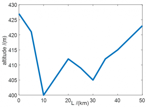
This research project is therefore devoted to the investigation of thermal insulation properties and fluid properties on the temperature profile in the pipeline system during steady state condition. The thermal insulation design should have a capability of maintaining the temperature above 40℃. This project is therefore restricted to: undulated subsea pipeline of 427m of altitude and 50km long; passive thermal insulation. This work contributes to a better understanding of the calculation of temperature and pressure distributions during gas and liquid flow in subsea pipeline using black oil model approach for fluids properties characterization, which lead to the optimal choice of the thermal insulation design.
This study is organized as follow: Section 2 presents the methodology and the propose algorithm for steady state flow analysis. Section 3 presents ours case study and field data. The results of our numerical analysis are presented and discussed. Section 4 conclude the work and presents recommendations and future work.
2.1 Geometrical parameters of pipeline and insulation materials
The subsea pipeline geometry considered in this study is the same as that presented by Duan et al. [4] for the example 1 case. Figure 1 below represent a vertical section of the considered offshore pipeline. The figure was represented with MATLAB software based on data from the schematic in ref. [4].
Table 1. Geometrical parameters of pipeline and insulation [4]
|
Internal diameter of pipeline (m) |
Outer diameter of pipeline (m) |
Thickness of pipeline (m) |
Length of pipeline (m) |
|
0.3112 |
0.3239 |
0.0127 |
50,000 |
The geometrical parameters of the pipeline and insulation materials as well as the thermophysical properties of insulation materials are given in Table 1 and Table 2.
Figure 1. Vertical sectional profile of the pipeline [4]
Table 2. Thermophysical properties of the insulation materials [11, 12]
|
Insulation materials |
Thermal conductivity (W/m K) |
Specific heat (Kj/Kg K) |
Density (Kg/m³) |
|
Calcium Silicate |
0.069 |
0.96 |
260 |
|
Polyurethane |
0.04 |
1400 |
45 |
|
Black Aerogel |
0.012 |
950 |
140 |
2.2 Fluids properties
The black oil model assumed that there are at most three distinct phase: Oil, gas and water. Water and oil are assumed to be immiscible and they do not exchange mass or change phase. Gas is assumed to be soluble in oil but not in water. In this work, the fluids properties were calculated using the black oil approached as follow. All black oil variables are given in S.I units unless precise.
2.2.1 Bubble point pressure Pb
The bubble point pressure can be determined by [13]:
$\mathrm{P}_{\mathrm{b}}=1.255\left[\left(\frac{\mathrm{GOR}}{0.0059 \gamma_{\mathrm{g}} 10^{2.14 / \mathrm{\gamma}_{\mathrm{o}} 10^{-0.00198 \mathrm{~T}}}}\right)^{0.83}-1.76\right]$ (1)
with T is in °k, Pb in Bar.
2.2.2 Gas oil solution Rs
Standing in 1951 [14], proposed a correlation for the calculation of the gas-oil solution.
$\mathrm{R}_{\mathrm{S}}=0.00590 \gamma_{\mathrm{g}} 10^{2.14 / \gamma \circ} 10^{-0.00198 \mathrm{~T}}\left(0.797 .10^{-5} \mathrm{P}+1.4\right)^{1.205}$ (2)
For pressures greater than bubble point pressure, Rs=GOR, with T in °k and P in Pa, Rs in Sm³/Sm³.
2.2.3 Oil formation volume factor Bo
Bo is defined as the ratio between the oil volume at flow conditions and the oil volume at standard conditions.
$\mathrm{B}_{\mathrm{o}}=\frac{\mathrm{V}_{\mathrm{o}}(\mathrm{P}, \mathrm{T})}{\mathrm{V}_{\mathrm{o}_{-}} \mathrm{SC}}=\frac{\mathrm{Q}_{\mathrm{o}}(\mathrm{P}, \mathrm{T})}{\mathrm{Q}_{\mathrm{o}_{-} \mathrm{sc}}}=\frac{\mathrm{V}_{\mathrm{so}}}{\mathrm{V}_{\mathrm{so}_{-} \mathrm{sc}}}$ (3)
Oil formation volume factors at or less than bubble point pressures can be estimated by using the correlation obtained by Standing [14].
$\mathrm{B}_{\mathrm{o}}=0.9759+0.952 .10^{-3}\left(\mathrm{R}_{\mathrm{s}}\left(\frac{\gamma_{\mathrm{g}}}{\gamma_{\mathrm{osc}}}\right)^{0,5}+0.401 \mathrm{~T}-103\right)^{1.2}$ (4)
For pressures greater than bubble point pressure, oil formation volume factor is calculated by [14]:
$B_{0}=B_{o b} \exp \left[-C_{0}\left(P-10^{5} P_{b}\right)\right]$ (5)
The coefficient of oil isothermal compressibility is calculated by Vazquez and Beggs [15] using the correlation below:
$C_{0}=10^{-9} \frac{2.81 \mathrm{Rs}+3.10 \mathrm{~T}+\frac{171}{\gamma_{\mathrm{o}}}-118 \gamma_{\mathrm{g}}-1102}{\mathrm{P}}$ (6)
With, T in °k, P in Bar, Bo in m³/m³ and Co in Bar-1.
2.2.4 Oil viscosity μo
The oil viscosity is determined for three thermodynamic pressure levels
$\mu_{o d}=C_{4}\left(0.32+\frac{1.8 \times 10^{7}}{A P I^{4.53}}\right)$
$\left(\frac{360}{C_{3}+200}\right)^{10^{\left(0.43+\frac{8.33}{A P I}\right)}}$ (7)
$\mu_{\mathrm{o}}=10.715 \mathrm{C}_{4}\left(\mathrm{C}_{1} \mathrm{Rs}+100\right)^{-0.515}\left(\frac{\mu_{\mathrm{od}}}{\mathrm{C}_{4}}\right)^{\left(5.44\left(\mathrm{C}_{1} \mathrm{Rs}+150\right)^{-0.338}\right)}$ (8)
$\mu_{\mathrm{o}}=\mu_{\mathrm{ob}}\left(\frac{\mathrm{P}}{\mathrm{P}_{\mathrm{b}}}\right)^{\mathrm{m}}$ (9)
where,
$\mathrm{m}=2.6\left(\mathrm{C}_{2} \mathrm{P}\right)^{1.187} \times \mathrm{e}^{-11.513-8.9810^{-5} \mathrm{C}_{2} \mathrm{P}}$ (10)
μob is the viscosity at the bubble-point pressure obtained using and setting Rs=GOR.
μo is given in Pa.s.
2.2.5 Oil specific gravity and oil density γo, ρo
In petroleum industry, the oil specific gravity and oil density are given by:
$\gamma_{\mathrm{o}}=\frac{141.5}{\mathrm{API}+131.5}$ (11)
$\rho_{\mathrm{o}_{-} \mathrm{sc}}=\gamma_{\mathrm{o}} \rho_{\mathrm{w}_{-} \mathrm{sc}}$ (12)
$\rho_{o}=\frac{\rho_{\mathrm{o}_{-} \mathrm{sc}}+\rho_{\mathrm{g}_{-}{\mathrm{s} \mathrm{c}}} \mathrm{R}_{\mathrm{s}}}{\mathrm{B}_{\mathrm{o}}}$ (13)
where,
ρo_sc, ρw_sc and ρg_sc are standard densities of oil, water and gas respectively. γo is the specific density of oil. ρo is the local density of oil at flow conditions.
2.2.6 Gas compressibility factor Z
Correlation presented by Andreolli et al. [11] approximating the abacus data in Standing and Katz [19] is given by:
$\mathrm{Z}=1-\frac{3.52}{10^{0.9813 \mathrm{~T} \mathrm{pr}}}+\frac{0.274 \mathrm{P}_{\mathrm{pr}}^{2}}{10^{0.8157 \mathrm{~T} \mathrm{pr}}}$ (14)
$\mathrm{T}_{\mathrm{pr}}=\frac{\mathrm{T}}{\mathrm{T}_{\mathrm{pc}}}$ (15)
$P_{p r}=\frac{P}{P_{p c}}$ (16)
where, the pseudocritical properties were calculated using the Standing [15] correlation
$\mathrm{T}_{\mathrm{pc}}=\frac{1}{\mathrm{C}_{5}}\left(168+325 \gamma_{\mathrm{g}}-12.5 \gamma_{\mathrm{g}}^{2}\right)$ (17)
$\mathrm{P}_{\mathrm{pc}}=\frac{1}{\mathrm{C}_{2}}\left(677+15.0 \gamma_{\mathrm{g}}-37.5 \gamma_{\mathrm{g}}^{2}\right)$ (18)
2.2.7 Gas formation volume factor Bg
Bg is defined by the ratio of the free gas volume in flow condition to the volume at standard condition of the same mass of gas.
$\mathrm{B}_{\mathrm{g}}=\frac{\mathrm{V}_{\mathrm{g}}(\mathrm{P}, \mathrm{T})}{\mathrm{V}_{\mathrm{g}_{-} \mathrm{sc}}}=\frac{\rho_{\mathrm{g}_{-} \mathrm{sc}}}{\rho_{\mathrm{g}}}$ (19)
$\mathrm{B}_{\mathrm{g}}=\frac{\mathrm{P}_{\mathrm{sc}}}{\mathrm{T}_{\mathrm{sc}}} \frac{\mathrm{ZT}}{\mathrm{P}}$ (20)
where, Psc and Tsc are pressure and temperature at standard condition. T and P are temperature and pressure at flow conditions respectively.
2.2.8 Gas density ρg
$\rho_{\mathrm{g}}=0.009225 \frac{\gamma_{\mathrm{g}} \mathrm{P}}{\mathrm{ZT}}$ (21)
where, T is in °k, P in Pa.
2.2.9 Gas viscosity μg
For the gas viscosity calculation, we used the Lee et al. [18].
$\mu_{\mathrm{g}}=\mathrm{C}_{4} \mathrm{~F}_{1} \exp \left(\mathrm{F}_{2}\left(\mathrm{C}_{4} \rho_{\mathrm{g}}\right)^{\mathrm{F}_{3}}\right)$ (22)
$\mathrm{F}_{1}=\frac{\left(9.379+16.07 \mathrm{M}_{\mathrm{g}}\right)\left(\mathrm{C}_{5} \mathrm{~T}\right)^{1.5}}{209.2+19260 \mathrm{M}_{\mathrm{g}}+\mathrm{C}_{5} \mathrm{~T}}$ (23)
$\mathrm{F}_{2}=3.448+\frac{986.4}{\mathrm{C}_{5} \mathrm{~T}}+10.09 \mathrm{M}_{\mathrm{g}}$ (24)
$\mathrm{F}_{3}=2.447-0.2224 \mathrm{~F}_{2}$ (25)
where, T is in °k
2.2.10 Water formation volume factor BW
BW is defined as the ratio between the water volume at flow conditions and the water volume at standard conditions.
$B_{\mathrm{w}}=\frac{\mathrm{V}_{\mathrm{w}}(\mathrm{P}, \mathrm{T})}{\mathrm{V}_{\mathrm{w}_{-} \mathrm{s} \mathrm{c}}}=\frac{\mathrm{Q}_{\mathrm{w}}(\mathrm{P}, \mathrm{T})}{\mathrm{Q}_{\mathrm{w}_{-} \mathrm{sc}}}$ (26)
It can be calculated using the McCain correlation [20].
$B_{W}=\left(1+\Delta V_{w T}\right)\left(1+\Delta V_{w P}\right)$ (27)
where, $\Delta V_{w T}$ and $\Delta V_{w P}$ are respectively the volume corrections for temperature and pressure, obtained by:
$\Delta \mathrm{V}_{\mathrm{wT}}=-1.00010\left(10^{-2}\right)+1.33391\left(10^{-4}\right) \mathrm{C}_{3}+5.50654\left(10^{-7}\right) \mathrm{C}_{3}^{2}$ (28)
$\begin{array}{rl}\Delta \mathrm{V}_{\mathrm{wP}}=-1.9530 1\left(10^{-9}\right) \mathrm{C}_{2} \mathrm{C}_{3} \mathrm{P} \\ & -1.72834\left(10^{-13}\right) \mathrm{C}_{2}{ }^{2} \mathrm{C}_{3} \mathrm{P}^{2} \\ & -3.58922\left(10^{-7}\right) \mathrm{C}_{2} \mathrm{P} \\ & -2.25341\left(10^{-10}\right) \mathrm{C}_{2}{ }^{2} \mathrm{P}^{2}\end{array}$ (29)
T is given in °k and P in Pa.
2.2.11 Water density
The water density at local flow condition is calculated as:
$\rho_{\mathrm{W}}=\frac{\rho_{\mathrm{w}_{-} \mathrm{sc}}}{\mathrm{B}_{\mathrm{w}}}$ (30)
where, ρwsc and γwsc are respectively water density at standard conditions and specific gravity of water at standard condition.
2.2.12 Water viscosity
The water viscosity was estimated by using the correlation of Collins [21], neglecting salinity effect as presented by [11].
$\mu_{\mathrm{w}_{\mathrm{sc}}}=109.574 \mathrm{C}_{4} \mathrm{C}_{3}^{-1.12166}$ (31)
$\mu_{\mathrm{w}}=\mu_{\mathrm{wsc}}\left(0.999+4.029510^{-5} \mathrm{k}_{6}+3.1062 \times 10^{-9} \mathrm{k}_{6}^{2}\right)$ (32)
$\mathrm{k}_{6}=\left(\mathrm{C}_{2} \mathrm{P}+14.7\right)$ (33)
2.2.13 Volumetric flow rate
Volumetric flow rate of petroleum fluids (gas, oil and water) at flow conditions are defined as follow:
Qg=(Qg_sc-RsQo_sc) Bg=Qo_sc(GOR-Rs) Bg (34)
Qo=Qo_scBo (35)
Qw=Qw_scBw (36)
Ql=Qo_scBo+Qw_scBw=Qo_sc(Bo+WOR.Bw) (37)
where, Qg_sc, Qw_sc and Qo_sc are the flow rates of gas, water and oil at standard conditions. Qg, Qw, Qo and Ql are the flow rates of gas, water, oil and liquid at flow conditions. GOR and WOR are gas oil ratio and water oil ratio at surface.
2.3 Pressure gradient formulation
The pressure gradient is calculated using Dukler and Taitel correlation [22] in which, void fraction is determined based on drift-flux model using correlations from [23]. Eq. (1) below describes the pressure profile along a flow-line.
$\left(\frac{\mathrm{dP}}{\mathrm{dL}}\right)=\frac{\mathrm{f}_{\mathrm{tp}} \rho_{\mathrm{m}} \mathrm{V}_{\mathrm{m}}^{2}}{2 \mathrm{D}}+\rho_{\mathrm{m}} g \sin (\theta)$ (38)
where: P is the pressure given in Pa; L is the length of the pipeline in m; ρm is the mixture local density in kg.m-3; vm is the mixture velocity in m.s-1; D is the pipeline outer diameter in m; g is the gravitational acceleration given in m.s-2 and θ is the inclinasion of the pipeline expressed in degrees. In Eq. (38), two necessary variables are to be determined: the friction factor of two-phase flow ftp and the mixture density ρm.
$\rho_{\mathrm{m}}=\rho_{\mathrm{L}}\left(\frac{\lambda^{2}}{1-\alpha}\right)+\rho_{\mathrm{g}}\left(\frac{(1-\lambda)^{2}}{\alpha}\right)$ (39)
$\frac{1}{\sqrt{f_{t p}}}=-2 \log \left[\frac{2 \varepsilon / d}{3.7}-\frac{5.02}{\operatorname{Re}} \log \left(\frac{2 \varepsilon / d}{3.7}+\frac{13}{R e}\right)\right]$ (40)
$\lambda=\frac{Q_{o_{-} s c} B_{o}+Q_{w_{-} s c} B_{w}}{Q_{o_{-} s c} B_{o}+Q_{w_{-} s c} B_{w}+\left(Q_{g_{-} s c}-Q_{o_{-} s c} R_{s}\right) B_{g}}$ (41)
$\alpha=\frac{\mathrm{V}_{\mathrm{sg}}}{\mathrm{C}_{\mathrm{d}} \mathrm{V} \mathrm{m}+\mathrm{V}_{\mathrm{d}}}$ (42)
$C_{d}=\frac{V_{s g}}{V_{m}}\left[1+\left(\frac{V_{s l}}{V_{s g}}\right)^{\left(\frac{\rho_{g}}{\rho_{L}}\right)^{0.1}}\right]$ (43)
$\mathrm{V}_{\mathrm{d}}=2.9\left[\frac{\mathrm{g} \cdot \mathrm{D} \cdot \sigma(1+\cos \theta)\left(\rho_{\mathrm{L}}-\rho_{\mathrm{g}}\right)}{\rho_{\mathrm{L}}^{2}}\right]^{0.25}(1.22+1.22 \sin \theta)^{\frac{\mathrm{P}_{\mathrm{atm}}}{\mathrm{P}}}$ (44)
From (Eq. (38)) to (Eq. (44)):
ρg, is the local density of the gas, kg.m-3; ρL is the local liquid density, kg.m-3; α is the void fraction of the gas phase given by drift flux correlation of Woldesemayat. For more details, see [23]. Vsg is the superficial velocity of the gas phase, m.s-1; Vm is the mixture velocity, m.s-1; Cd is the profile parameter and Vd is the drift velocity. σ is the surface tension calculated given in N.m-1. Patm, is the atmospheric pressure, in Pa. λ is the liquid input fraction. Qo_sc and Qw_sc are oil and water flowrate respectively at standard condition given in m3.s-1. Black oil parameters which are: Bw, m3.s-3; Bg, m3.m-3; Bo, m3.m-3; Rs, Sm3.Sm-3, ε, is the pipe roughness, d the pipe diameter and Re is the Reynolds number of the mixture given by (Eq. (45)) below:
$\mathrm{Re}=\frac{\rho_{\mathrm{m}} \mathrm{V}_{\mathrm{m}} \mathrm{d}}{\mu_{\mathrm{m}}}$ (45)
2.4 Temperature profile model using MATLAB
Difference material of thermal insulation will result to various temperature profile inside the subsea pipeline. Thus, we present here the temperature calculations model for an oil and gas flow inside subsea pipeline. The temperature are pressure dependent. From the general equation describing the temperature profile along pipeline considering that the kinetic energy is negligible as in ref. [24], we have:
$\begin{aligned} \frac{\partial\left(\mathrm{T}_{\mathrm{m}}\right)}{\partial \mathrm{t}}-\eta_{\mathrm{m}} \frac{\partial \mathrm{P}}{\partial \mathrm{t}}=&-\mathrm{v}_{\mathrm{m}} \frac{\partial\left(\mathrm{T}_{\mathrm{m}}\right)}{\partial \mathrm{L}}-\frac{\mathrm{U}_{\mathrm{o}} \pi \mathrm{D}\left(\mathrm{T}_{\mathrm{m}}-\mathrm{T}_{\mathrm{e}}\right)}{\mathrm{A}_{\mathrm{p}} \rho_{\mathrm{m}} \mathrm{Cp}_{\mathrm{m}}} \\ &+\mathrm{v}_{\mathrm{m}} \eta_{\mathrm{m}} \frac{\partial \mathrm{P}}{\partial \mathrm{L}}-\mathrm{v}_{\mathrm{m}} \frac{\mathrm{g} \sin (\theta)}{\mathrm{C}_{\mathrm{p}_{\mathrm{m}}}} \end{aligned}$ (46)
where, Tm is the average temperature of the fluid given in °k, Ap is the pipe cross-sectional area m2, t is the time given in $C_{p_{m}}$ is the mixture specific heat capacity in J.k.kg-1, ηm is the mixture Joule Thomson coefficient, k.Pa-1, Uo is the overall heat transfer coefficient in w.k.m-2, Te is the environment temperature in °k.
In steady state conditions, (Eq. (47)) becomes:
$\frac{\mathrm{dT}_{\mathrm{m}}}{\mathrm{dL}}=-\frac{\mathrm{U}_{\mathrm{o}} \pi \mathrm{D}\left(\mathrm{T}_{\mathrm{m}}-\mathrm{T}_{\mathrm{e}}\right)}{\mathrm{C}_{\mathrm{p}_{\mathrm{m}}} \mathrm{w}_{\mathrm{m}}}+\eta_{\mathrm{m}} \frac{\mathrm{dP}}{\mathrm{dL}}-\frac{\mathrm{g} \sin (\theta)}{\mathrm{C}_{\mathrm{p}_{\mathrm{m}}}}$ (47)
where:
$\mathrm{w}_{\mathrm{m}}=\rho_{\mathrm{m}} \mathrm{V}_{\mathrm{m}} \mathrm{A}_{\mathrm{p}}$ (48)
$\mathrm{Cp}_{\mathrm{m}}=\mathrm{Cp}_{\mathrm{g}} \alpha \frac{\rho_{\mathrm{g}}}{\rho_{\mathrm{m}}}+\mathrm{Cp}_{\mathrm{L}}(1-\alpha) \frac{\rho_{\mathrm{L}}}{\rho_{\mathrm{m}}}$ (49)
$\mathrm{Cp}_{\mathrm{L}}=\left(\frac{\mathrm{Q}_{\mathrm{o}}}{\mathrm{Q}_{0}+\mathrm{Q}_{\mathrm{w}}}\right) \mathrm{Cp}_{\mathrm{o}}+\left(\frac{\mathrm{Q}_{\mathrm{w}}}{\mathrm{Q}_{0}+\mathrm{Q}_{\mathrm{w}}}\right) \mathrm{Cp}_{\mathrm{w}}$ (50)
From (Eq. (47) to (Eq. (50)):
$w_{m}$ is the mixture mass flow rate in kg.s, Cpm, is the average specific heat capacity calculated as in ref. [25], Cpg and CpL are the specific heat capacity of the gas and liquid respectively. Cpm, Cpg and CpL are expressed in J.k.kg-1. Qo and Qw are respectively the local flowrates of the oil and water. ηm, is the average Joule-Thomson, coefficient calculated using (Eq. (51)) through (Eq. (54)) as shown below,
$\eta_{\mathrm{m}}=-\left(\frac{\mathrm{w}_{\mathrm{g}} \mathrm{Cp}_{\mathrm{g}} \eta_{\mathrm{g}}+\mathrm{w}_{\mathrm{L}} \mathrm{Cp}_{\mathrm{L}} \eta_{\mathrm{L}}}{\mathrm{w}_{\mathrm{m}} \mathrm{Cp}_{\mathrm{m}}}\right)$ (51)
$\eta_{\mathrm{g}}=\left(\frac{1}{\rho_{\mathrm{g}} \mathrm{C}_{\mathrm{p}} \mathrm{g}}\right)\left[\frac{\mathrm{T}_{\mathrm{m}}}{\mathrm{Z}}\left(\frac{\mathrm{dZ}}{\mathrm{dT}}\right)_{\mathrm{p}}\right]$ (52)
$\eta_{\mathrm{L}}=\frac{1}{\rho_{\mathrm{L}} \mathrm{Cp}_{\mathrm{L}}}\left(\mathrm{T}_{\mathrm{m}} \beta-1\right)$ (53)
$\beta=\frac{\mathrm{WOR}}{1+\mathrm{WOR}} \frac{\partial \mathrm{B}_{\mathrm{w}}}{\partial \mathrm{T}}+\frac{1}{1+\mathrm{WOR}} \frac{\partial \mathrm{B}_{\mathrm{o}}}{\partial \mathrm{T}}$ (54)
Where is the thermal expansion coefficient and Z is the gas compressible factor.
The overall heat transfer coefficient Uo is calculated as
$\frac{1}{\mathrm{U}_{\mathrm{o}}}=\left(\frac{\mathrm{r}_{\mathrm{ins}}}{\mathrm{r}_{\mathrm{i}} \mathrm{h}_{\mathrm{in}}}+\mathrm{r}_{\mathrm{ins}} \frac{\ln \left(\frac{\mathrm{r}_{\mathrm{o}}}{\mathrm{r}_{\mathrm{i}}}\right)}{\mathrm{k}_{\mathrm{pipe}}}+\mathrm{r}_{\mathrm{ins}} \frac{\ln \left(\frac{\mathrm{r}_{\mathrm{ins}}}{\mathrm{r}_{\mathrm{o}}}\right)}{\mathrm{k}_{\mathrm{ins}}}+\frac{\mathrm{r}_{\mathrm{ins}}}{\mathrm{h}_{\mathrm{o}}}\right)$ (55)
kpipe and kins represent the thermal conductivity of the metallic pipe and the insulation layer respectively, they are expressed in, w.k-1.m-1. rins, ro and ri are respectively the insulation material radius, the outer and the inner radius given in m. The surrounding heat transfer coefficient ho expressed in w.k-1.m-2, is calculated using (Eq. (56)) below:
$h_{0}=\frac{K_{0} N u_{0}}{D}$ (56)
where, $N u_{o}=0.027 . R_{e o}^{0.8} P_{r o}^{0.3}$, represent the Nusselt number; $R e_{o}=\frac{\rho_{o} V_{o} D}{\mu_{o}}$, is the outer Reynolds number of the seawater; ρo is the density of the seawater, kg.m-3; Vo, is the seawater velocity, m/s; μo is the viscosity of the seawater, in Pa.s;
$P r_{o}=\frac{\mu_{o} C p_{o}}{K_{o}}$, is the Prandtl number of the outer seawater; Cpo is the specific heat capacity of the seawater, J.k.kg-1; Ko is the thermal conductivity of the seawater, w.k-1.m-1.
The internal heat transfer coefficient expressed in w.k-1.m-2, is calculated according to Pourafshary et al. [25] as follow:
$h_{\text {in }}=\frac{K_{\text {tp }} N u_{\text {tp }}}{D}$ (57)
where, Ktp expressed in w.k-1.m-1, is the mixture thermal conductivity of the two-phase flow given as
$\mathrm{K}_{\mathrm{tp}}=\alpha \mathrm{k}_{\mathrm{g}}+(1-\alpha) \mathrm{k}_{\mathrm{L}}$ (58)
With kg and kL representing each the thermal conductivity of the gas and liquid respectively, expressed both in w.k-1.m-1.
Nutp, the Nusselt number of the two-phase flow determined as follow:
If flow is laminar (ReT≤2000), for long pipe, we have:
$\mathrm{Nu}_{\mathrm{tp}}=1.86\left[\mathrm{Re}_{\mathrm{T}} \operatorname{Pr}_{\mathrm{m}}\left(\frac{\mathrm{D}}{\mathrm{L}}\right)\right]^{\frac{1}{3}}$ (59)
If flow is turbulent flow (ReT≥6000), for long pipe, we have:
$\mathrm{Nu}_{\mathrm{tp}}=0.023 \mathrm{Re}_{\mathrm{T}}^{0.8} \operatorname{Pr}_{\mathrm{m}}^{0.33}\left(1+\left(\frac{\mathrm{D}}{\mathrm{L}}\right)^{0.7}\right)$ (60)
For transition flow regime (2000≤ReT≤6000)
$\mathrm{Nu}_{\mathrm{tp}}=\mathrm{Nu}_{\text {laminar }}\left[\frac{\mathrm{Re}_{\mathrm{T}}}{6000}\right]^{\mathrm{a}}$ (61)
with, parameter a given by:
$\mathrm{a}=\frac{\ln \left(\frac{\mathrm{Nu}_{\text {turbulent }}}{\mathrm{Nu}_{\text {laminar }}}\right)}{\ln \left(\frac{\mathrm{Re}_{\mathrm{max}}}{\mathrm{Re}_{\min }}\right)}$ (62)
The total Reynolds number ReT is calculated as follow:
$\mathrm{Re}_{\mathrm{T}}=\frac{\rho_{\mathrm{L}} \mathrm{V}_{\mathrm{sL}} \mathrm{D}}{\mu_{\mathrm{L}}}+\frac{\rho_{\mathrm{g}} \mathrm{V}_{\mathrm{sg}} \mathrm{D}}{\mu_{\mathrm{g}}}$ (63)
The Prandtl number of the mixture is given by:
$\operatorname{Pr}_{\mathrm{m}}=\frac{\mu_{\mathrm{m}} \mathrm{Cp}_{\mathrm{m}}}{\mathrm{K}_{\mathrm{tp}}}$ (64)
2.5 Numerical simulations
The finite difference method was used to discretize the temperature model given by Eq. (47). All the equations in this study are solved simultaneously using MATLAB software. Numerically, we divide the pipeline into sections, and each section was divided into cells and consider average value of temperature and pressure in the cells. The numerical solution obtained using finite difference method is therefore given by:
$\frac{\mathrm{T}_{\mathrm{m}}(\mathrm{i}+1)-\mathrm{T}_{\mathrm{m}}(\mathrm{i})}{\Delta \mathrm{x}}=\left(\frac{\mathrm{T}_{\mathrm{e}}-\mathrm{T}_{\mathrm{m}}}{\mathrm{A}}+\eta_{\mathrm{m}} \frac{\mathrm{dP}}{\mathrm{dL}}-\frac{\mathrm{g} \sin (\theta)}{\mathrm{C}_{\mathrm{p}_{\mathrm{m}}}}\right)_{\mathrm{i}}$ (65)
In which, the parameter A is:
$A_{i}=\left(\frac{C_{p_{m}} w_{m}}{U_{0} \pi D}\right)_{i}$ (66)
The temperature model presented above is first validated by using it to produce the same work done by [4]. The difference done here by this research is the methodology approach for the determination of the pressure gradient, the calculation of the Z-factor, the calculation of the liquid holdup and the determination of the of the joule Thomson coefficient of gas, liquid and thus, for the mixture. In Table 3 below, we present all the necessary inputs fluids data to run simulations.
Table 3. Operating parameters [4]
|
Oil flow rate |
0.00955m³/s |
|
Gas flow rate |
9.05 Nm³ |
|
Density of natural gas |
0.710 Kg/m³ |
|
Density of crude oil (20℃) |
886.9 Kg/m³ |
|
Surrounding temperature |
277.15 K |
|
Inlet temperature |
323.15 K |
|
Outlet temperature |
278.75 K |
|
Inlet pressure |
5 MPa |
|
Outlet pressure |
2.4 MPa |
|
Over all heat transfer coefficient |
2 (W/m² K) |
2.6 Temperature model using PIPESIM
This study also uses the PIPESIM software to build and validate the temperature model presented above. The operating parameters are enter in the software. The fluid type is set as black oil. The simulations are
2.6.1 Pipeline model
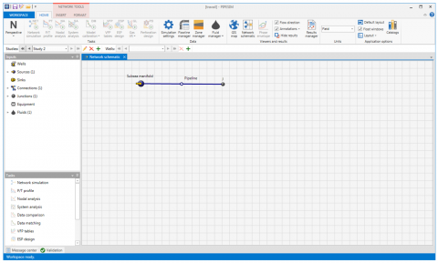
The network schematic model was used to build the pipeline model in PIPESIM. Figure 2 below shows a sketch of the simulation modeling of the pipeline in PIPESIM.
2.6.2 Multiphase correlation
The multiphase model selected in PIPESIM was the revised correlation of Beggs and Brill [17] described by the following equation
$\frac{d P}{d L}=\frac{\frac{f_{t p} \rho_{n V_{m}^{2}}}{2 d}+\rho_{m} g \sin \theta}{1-E_{k}}$ (67)
In which $E_{k}$ is a dimensionless acceleration term that take into consideration the pressure gradient due to kinetic energy effects and is given by:
$\mathrm{E}_{\mathrm{k}}=\frac{\mathrm{V}_{\mathrm{m}} \mathrm{V}_{\mathrm{Sg}} \rho_{\mathrm{m}}}{\mathrm{P}}$ (68)
The Beggs and Brill multiphase correlation deals with both the friction pressure loss and the hydrostatic pressure difference. First the appropriate flow regime for the particular combination of gas and liquid rates (Segregated, Intermittent or Distributed) is determined. The liquid holdup, and hence, the in-situ density of the gas-liquid mixture is then calculated according to the appropriate flow regime, to obtain the hydrostatic pressure difference. A two-phase friction factor is calculated based on the "input" gas-liquid ratio and the Moody friction factor table using Colebrook equation. From this, the friction pressure loss is calculated using "input" gas-liquid mixture properties. That is why this model was selected.
Figure 2. Sketch of the simulation modeling of subsea pipeline in PIPESIM
2.6.3 Energy equation
PIPESIM uses the first law of thermodynamics to perform a rigorous heat transfer balance on each pipe segment. The first law of thermodynamics is the mathematical formulation of the principle of conservation of energy applied to a process occurring in a closed system (a system of constant mass m). It equates the total energy change of the system to the sum of the heat added to the system and the work done by the system. For steady-state flow, it connects the change in properties between the streams flowing into and out of an arbitrary control volume (pipe segment) with the heat and work quantities across the boundaries of the control volume (pipe segment). For a multiphase fluid in steady-state flow, the energy equation is given by:
$\Delta\left[\left(\mathrm{H}+\frac{1}{2} \mathrm{~V}_{\mathrm{m}}^{2}+\mathrm{gz}\right) \mathrm{dm}\right]=\sum \delta \mathrm{Q}-\delta \mathrm{W}$ (69)
where the specific enthalpy:
H=U+PV (70)
is a state property of the system since the internal energy U the pressure P and the volume V are state properties of the system.
It is clear from the left-hand side of Eq. (69), the change in total energy is the sum of the change in enthalpy energy,
$\Delta[\mathrm{Hdm}]=\Delta[(\mathrm{U}+\mathrm{PV}) \mathrm{dm}]$ (71)
the change in gravitational potential energy:
$\Delta\left(\mathrm{E}_{\mathrm{p}}\right)=\Delta[(\mathrm{gz}) \mathrm{dm}]$ (72)
and the change in total kinetic energy (based on the mixture velocity)
$\Delta\left(\mathrm{E}_{\mathrm{k}}\right)=\Delta\left[\left(\frac{1}{2} \mathrm{~V}_{\mathrm{m}}^{2}\right) \mathrm{d} \mathrm{m}\right]$ (73)
which is assumed to be negligible.
On the right-hand side of Eq. (69), ∑δQ includes all the heat transferred to the control volume (pipe segment) and δW represents the shaft work, that is work transmitted across the boundaries of the control volume (pipe segment) by a rotating or reciprocating shaft
2.6.4 Setup calculation
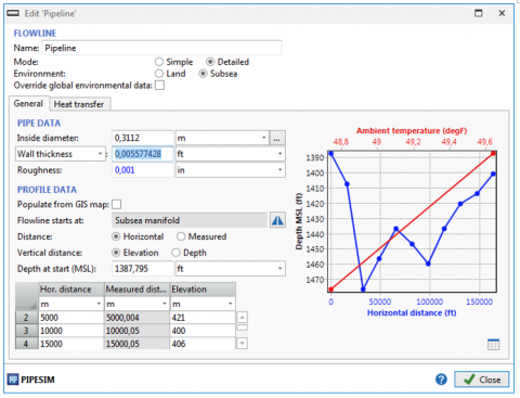
In PIPESIM, after the pipeline model is built and the fluid model is considered, the setup data for simulations can then be edited as it be seen in the Figure 3 below.
Figure 3. Sketch of data edit in PIPESIM
2.6.5 Run simulations
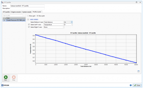
You can perform nodal analysis, reservoir simulation, and use other analytical tools (such as pressure/temperature (P/T) profiles, VFP tables, and network simulation) to calculate the distribution of flowrates, temperatures, and pressures throughout the system and plan new field developments. Figure 4 below presents a sketch of temperature simulation run using PIPESIM.
Figure 4. Sketch of temperature simulation with PIPESIM
The given calculations are performed to select the insulation material and appropriate insulation layer thickness. The design criterion is to ensure that the temperature at any point on the flow line does not drop to below 40℃, as required by flow assurance. Insulating materials considered for this design are Calcium Silicate (CS), Black Aerogel (BA) and Polyurethane Foam (PUF). Firstly, MATLAB software was used to implement numerical simulations and PIPESIM software was used for numerical validation purpose of the temperature profile. Further simulations are run to thermally design the subsea pipeline. Finally, the effect of the selected insulation material on the heat flux and the phase envelop of the fluids was carried out
3.1 Pressure profile inside the subsea pipeline
As pressure and temperature are simultaneously dependent, we first present the result of the pressure profile along the considered subsea pipeline. In order to verify the pressure model describes above in Eq. (38), numerical simulation was performed with MATLAB software using data presented in Table 3 above. The validation of the predicted model is done using PIPESIM software and measure value data obtained from [4].
3.1.1 Validation with the PIPESIM model
In order to validate the model used for predicting the pressure profile, the output of the predicted model was compared to the output of the PIPESIM model. From Figure 5 above, we observed the Pressure drop is not linear because of the presence of more than phase. Predicted pressure decreases along the subsea pipeline from 5×10⁶ Pa to 2.4327×10⁶ Pa. The pressure obtained with the PIPESIM software have an end-point value of 3×10⁶ Pa. The predicted used Dukler and Taitel model in which liquid holdup is calculated using drift-flux correlation while the PIPESIM model used the Beggs and Brill correlation. These different approaches could explain the difference observed when comparing the outputs of the models. However, the pressure drop from PIPESIM is closed to the one obtained by our predicted program with a relative error of about (3-2.4327)/3=19%. This shows that the predicted model presented in this study can be used for two-phase pressure drop calculation in an undulated subsea pipeline of about 50km. A greater pressure drop will cause a smaller displacement of the fluid, thus additional energy will be required to displace the fluid.
Figure 5. Pressure profile inside subsea pipeline obtained using proposed model with MATLAB software and validated with PIPESIM model
Table 4. Pressure comparison and validation [4]
|
Methods |
Inlet pressure/ (MPa) |
Endpoint pressure/ (MPa) |
Pressure drop /(MPa) |
REPD |
|
Model |
5 |
2.4327 |
2.5673 |
1.26% |
|
Measured Value |
5 |
2.4 |
2.6 |
|
3.1.2 Validation with measured data
We compared in Table 4, the end-point value of the predicted model of pressure profile and the measured value from experiment in [4]. We then calculated the relative pressure difference (REPD). From Table 4, we noticed that the predicted pressure and the measured end-value are in good agreement with a relative error of 1.26% which shows that the proposed model capture well the two-phase flow pressure profile inside the subsea pipeline.
3.2 Temperature profile inside subsea pipeline
Temperature is one of the most important parameter in all thermal insulation design in subsea pipeline. Before investigating on the proper insulation material and the required insulation thickness, the temperature profile of the fluid flowing inside the pipeline must be well described. In order to make sure that the proposed temperature model is good for further simulations run, validation was carried out using PIPESIM model, measured value from experiment in [4] and literature calculation model from [4]. The predicted temperature from Eq. (65) was implement in MATLAB.
3.2.1 Validation with the PIPESIM model
Using the data presented in Table 3 above in conjunction with the above temperature model described by Eq. (65), the predicted temperature profile has been calculated using MATLAB software. The model was first validated numerically with the PIPESIM software as shown in Figure 6 below. It can be observed that the mixture of oil and gas enters the subsea pipeline with a temperature of 323.15°k and decreases along the subsea pipeline until it reaches the temperature of approximately 277.9934°k. This result was obtained for an overall heat transfer coefficient U = 2 W/(m² K) as presented by Duan et al. [4]. From the plot, it can be observed that the predicted model and the PIPESIM model show a good agreement. It can also be observed that the flowing temperature decreases rapidly to 313.15°K for a travelled distance of about 0.5 km, which represent the maximum distance the fluid moved before starting undergoing flow assurance issues such as paraffin wax formation and deposition. By considering the pipeline length of 50 km, the close match results shows that the model can predict the temperature distribution of an oil and gas flow through an undulated subsea pipeline.
Figure 6. Temperature profile comparison between our model and PIPESIM model
Figure 7. Oil viscosity variation with temperature
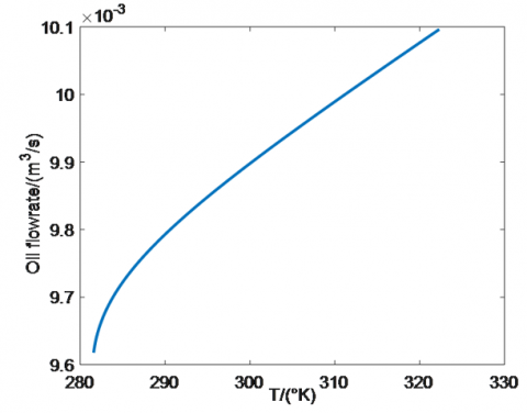
As the fluid temperature decreases along the pipeline due to the heat losses between the cold surrounding and the hot fluid, oil viscosity will increase as it is shown in Figure 7 above. Such situation may promote formation of solids such as wax in the pipeline resulting in pipeline obstruction thus to an increase in pressure drop of the fluid. Another problem, is the decrease of the oil production along the subsea production pipeline as can be seen in the Figure 8.
Figures 6, 7 and 8 show that the temperature is an important parameter for the analysis of fluid flow in subsea pipeline. A drop in temperature will cause a reduction in production due to a restriction of the flow area by solids deposition such as wax and hydrates resulting from a thermal unbalance between the surrounding cold water and the hot fluid flowing through the pipeline. This situation may required a more suitable insulation design for remediation.
Figure 8. Oil flowrate variation with temperature
3.2.2 Validation with measured field data from literature model
The model was also validated using measured value from field data. The results was presented and compared in Table 5 below. From this table, it is show that the predicted temperature from our model is in good agreement with that of the measured value and the predicted model from [4]. The results show a relative error of 1.68% with the measured value, 1.04% with the PIPESIM model and 3.37% with the model presented by Duan et al. [4]. This result shows that the model can predict accurately the temperature profile inside the considered subsea pipeline for an overall heat transfer coefficient U = 2 W/(m² K).
Table 5. Validation of the temperature calculations with others models
|
Methods |
Inlet temperature/(K) |
Endpoint temperature/(K) |
Temperature drop |
RETD |
|
Predicted model |
323.15 |
277.99 |
45.1566 |
1.68% |
|
MV |
323.15 |
278.75 |
44.4 |
1.04% |
|
PIPESIM prediction |
323.15 |
278.28 |
44.86 |
|
|
UPTP |
323.15 |
277.25 |
45.9 |
3.37% |
Form the results presented in Figure 6 and Table 5 above, it clear that the temperature model presented in this study can be further used for the thermal insulation design because of its good accuracy with other models. The main goal of the thermal design analysis was to select an appropriate insulation layer thickness and material. The design criterion is to ensure that the temperature at any point on the flow line does not drop to below 40℃, as required by flow assurance. Insulation materials considered for this design are Calcium Silicate, Polyurethane Foam and Black Aerogel.
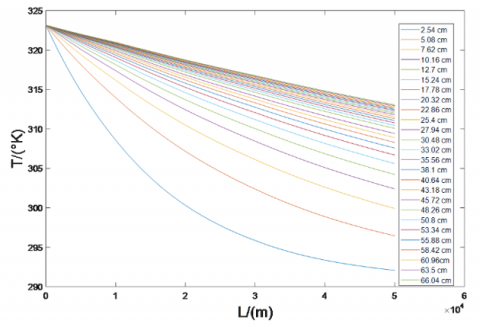
3.3 Numerical simulations for the determination of the minimum insulation thickness of Calcium Silicate
Figure 9 below shows the effect of various Calcium Silicate thickness on the fluid temperature along the subsea pipeline.
The thickness is comprised between 2.54 to 66.04 cm. It can be seen that, for insulation thickness less than 66.04 cm, the fluid temperature would drop below the 313.15°K, leading to high risk of flow assurance issues inside the subsea pipeline. The minimum insulation thickness to be used in this case is 66.04 cm.
Figure 9. Temperature profiles of the flowing fluids inside subsea pipeline with different insulation thickness of Calcium Silicate
3.4 Numerical simulations for the determination of the minimum insulation thickness of Polyurethane Foam
Figure 10 below, shows the temperature profile for different Polyurethane Foam thickness taken between 2.54 cm and 25.4cm. It can be observed that the minimum insulation thickness that would achieved an output temperature of at least 313.15°K is 25.4cm.
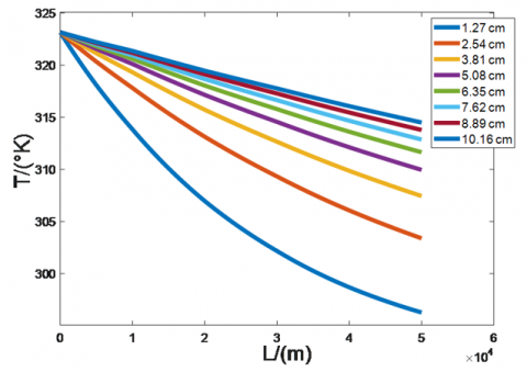
3.5 Numerical simulations for the determination of the minimum insulation thickness of Black Aerogel
In Figure 11 below, we plotted the temperature profile for different insulation thickness of Black Aerogel. The thickness range from 1.27 cm and 10.16 cm. The minimum insulation thickness necessary to satisfy the design criterion is 10.16 cm as can be seen.
When comparing the temperature profiles plotted in figure 9 to Figure 11 for the various insulating materials with different thickness, we observed that either a 25.4 cm of Polyurethane or a 10.16cm of Black Aerogel material should be used as insulating material type for the subsea pipeline. However, only cost analyses can justify one of the options, which is beyond the scope of this work. In this study, because Black Aerogel has the smallest thermal conductivity and provide the smallest insulation thickness, it was chosen as the best insulating material with a thickness of 10.16cm for the design purpose.
Figure 10. Temperature profiles of the flowing fluids inside subsea pipeline with different insulation thickness of Polyurethane Foam
Figure 11. Temperature profiles of the flowing fluids inside subsea pipeline with different insulation thickness of Black Aerogel
The temperature profiles have also help us to investigate the risk of flow assurance issues by examined the phase envelop.
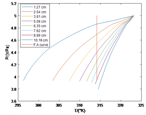
3.6 Effect of Black Aerogel on the phase diagram
Due to the low temperature and high pressure of deep water, the pipe thermal insulation has important effects on the fluid temperature in pipeline. Effect of Black Aerogel on the formation area of some flow assurance issues under different insulating material thickness.
In Figure 12, F.A is for Flow Assurance. The effect of different insulating material thickness was investigated on the phase diagram. It can be seen that the flow assurance risk formation area decreases with the increase of the thickness of insulating material. Thus, this approach can also be used to optimize the thermal insulation design of subsea pipeline.
Figure 12. Pressure variation vs temperature
In this work, we proposed a model to thermally design a subsea pipeline for heat conservation purpose in subsea pipeline and therefore to avoid the formation of some flow assurance issues such as paraffin wax and hydrates. As temperature and pressure greatly influence the flow assurance issues caused by thermal unbalance, a temperature and pressure model were proposed and validated using field data and others models. The good agreement obtained shows that the predicted models are suitable for temperature and pressure prediction in subsea pipeline. Further simulations were run to find out the optimal insulation thickness among three different insulating materials with various thicknesses in order to achieve the subsea pipeline design. From the obtained results, it is concluded that a minimum of 10.16 cm Black Aerogel thermal insulation thickness is required to ensure that the discharge temperature at the discharge end of the subsea pipeline does not fall below 313.15 degree Kelvin. It was also observed that, the selected insulation material has direct impacts on the flow assurance issues formation area in the subsea pipeline. Because of this, flow assurance risk formation region can be shifted or avoided. The proposed model can therefore be used to thermally design a subsea pipeline during steady state operation. For future work, logistic regression can be used to predict hydrate formation probability in a subsea production and transportation pipeline for a given composition and operating conditions. Machine learning approach can also be used to risk assessment of hydrate and wax formation. Multi-variate Logistic Regression Model to Analyze hydrate formation risk can also be carried out. Thermal insulation design can be studied on transporting pipeline that crosses offshore and onshore pipeline. Transient analysis can also be considered to capture wax, hydrates deposition tendencies during shut down, and restart scenarios for subsea pipeline transporting liquid and gas flow. A comparative study using PIPESIM, Aspen Hysys and MATLAB can be done in order to choose the best software that properly offer a good estimation of optimal insulation thickness. Investigation should be carried out for optimal economic insulation thickness design in subsea pipeline.
Thanks to the director of Environmental Energy Technologies Laboratory (E.E.T.L) for his time, counseling, guidance and availability.
|
A |
cross section area, m2 |
|
Bo |
oil formation volume factor, m3 .m-3 |
|
Bw |
water formation volume factor, m3 .m-3 |
|
Bg |
gas formation volume factor, m3 .m-3 |
|
Cd |
profile parameter |
|
Cp |
specific heat at constant pressure, $\mathrm{J} \cdot \mathrm{k}_{\mathrm{g}}^{-1} \cdot \mathrm{k}^{-1}$ |
|
D |
inner diameter of pipe, m |
|
f |
friction factor |
|
g |
acceleration of gravity, $\mathrm{m} \cdot \mathrm{s}^{-2}$ |
|
hin |
inner convective heat transfer coefficient, w. $k^{-1} . m^{-2}$ |
|
ho |
outer convection heat transfer coefficient, w. $k^{-1} . m^{-2}$ |
|
k |
thermal conductivity of pipe, w. $k^{-1} . m^{-1}$ |
|
L |
pipe length, m |
|
P |
pressure, Pa |
|
q |
heat flux rate |
|
Qw |
local flow rate of water at flow conditions, $\mathrm{m}^{3} \cdot \mathrm{s}^{-1}$ |
|
Qo |
local flow rate of oil at flow conditions, $\mathrm{m}^{3} \cdot \mathrm{s}^{-1}$ |
|
Qg |
local flow rate of gas at flow conditions, $\mathrm{m}^{3} \cdot \mathrm{s}^{-1}$ |
|
Qw_sc |
flow rate of water at standard conditions, $\mathrm{m}^{3} \cdot \mathrm{s}^{-1}$ |
|
Qo_sc |
flow rate of water at standard conditions, $\mathrm{m}^{3} \cdot \mathrm{s}^{-1}$ |
|
Qg_sc |
flow rate of water at standard conditions, $\mathrm{m}^{3} \cdot \mathrm{s}^{-1}$ |
|
Re |
Reynolds number |
|
RS |
solution gas-oil ratio, $\mathrm{Sm}^{3} . \mathrm{Sm}^{-3}$ |
|
r |
radius of pipe, m |
|
T |
temperature, k |
|
U |
overall heat transfer coefficient, w. $\mathrm{k} . \mathrm{m}^{-2}$ |
|
Vd |
drift velocity, $m . \mathrm{s}^{-1}$ |
|
Vsw |
superficial velocity of water, $m . \mathrm{s}^{-1}$ |
|
Vso |
superficial velocity of oil, $m . \mathrm{s}^{-1}$ |
|
Vsg |
superficial velocity of gas, $m . \mathrm{s}^{-1}$ |
|
Vg |
velocity of the gas phase, $m . \mathrm{s}^{-1}$ |
|
Vl |
velocity of the liquid phase, $m . \mathrm{s}^{-1}$ |
|
Vm |
mixture velocity, $m . \mathrm{s}^{-1}$ |
|
w |
mass flow rate, $\mathrm{k}_{\mathrm{g}} \cdot \mathrm{s}^{-1}$ |
|
Z |
gas compressibility factor |
|
Greek symbols |
|
|
ρ |
density, $\mathrm{k}_{\mathrm{g}} . \mathrm{m}^{-3}$ |
|
μ |
viscosity, kg. m-1.s-1 |
|
α |
void fraction |
|
η |
joule Thomson coefficient, $\mathrm{k} . \mathrm{Pa}^{-1}$ |
|
θ |
inclinasion angle of pipe, rad |
|
σ |
surface tension, $\mathrm{N} \cdot \mathrm{m}^{-1}$ |
|
Subscripts |
|
|
atm |
atmospheric |
|
o |
oil, outer |
|
g |
gas |
|
w |
water |
|
l |
liquid |
|
m |
mixture |
|
sc |
standard conditions |
|
tp |
two phase |
|
p |
pipe |
|
i |
inner |
|
ins |
insulation |
|
e |
ambient |
[1] Phil, H. (2007). Oil and Gas Pipelines: Yesterday and Today. International Petroleum Technology Institute, ASME, New York.
[2] Guo, B.Y. (2007). Petroleum Production Engineering: A Computer-Assited Approach. 1st (Ed.), Elsevier Science & Technology Books.
[3] Ahmed, I.M. (2018). Modeling and development of insulation materials in subsea. Master thesis, University of Newfoundland.
[4] Duan, J.M., Wang, W., Zhang, Y., Zheng, L.J., Liu, H.S., Gong, J. (2013). Energy equation derivation of the oil-gas flow in pipelines. Oil & Gas Science and Technology – Rev. IFP Energies Nouvelles, 68(2): 341-353. https://doi.org/10.2516/ogst/2012020
[5] Zulkefli, N.H.B., Pao, W. (2016). Optimum thermal insulation design for subsea pipeline flow assurance. Report number: 17276Affiliation: Universiti Teknologi PETRONAS. https://doi.org/10.13140/RG.2.2.33853.05603
[6] Patil, K.D., Sadafule, S. (2014). Study on effect of insulation design on thermal-hydraulic analysis: an important aspect in subsea pipeline designing. Technical Report, Maharashtra Institute of Technology, 4(1). https://www.researchgate.net/publication/263426807.
[7] Briggs, T.A., Onyegiri, I.E., Ekwe, E.B. (2020). Investigation of the effects of flowline sizes, flow rates, insulation material, type and configuration on flow assurance of waxy crude. Innovative Systems Design and Engineering, 11(3). https://doi.org/10.7176/ISDE/11-3-02
[8] Abegunde, M., Adeyemi, A. (2020). Optimisation of thermal insulation of subsea flowlines for hydrates. Society of Petroleum Engineers. https://doi.org/10.2118/203721-MS
[9] Marfo, S.A., Opoku Appau, P., Kpami, L.A.A. (2018). Subsea pipeline design for natural gas transportation: A case study of côte d’ivoire’s gazelle field. International Journal of Petroleum and Petrochemical Engineering (IJPPE), 4(3): 21-34. http://dx.doi.org/10.20431/2454-7980.0403003
[10] Alade, O. (2018). Sizing surface production flow line insulation thickness for a desired output temperature. Petroleum & Petrochemical Engineering Journal, 2(7). https://doi.org/10.23880/ppej-16000178
[11] Andreolli, I., Zortea, M., Baliño, J.L. (2017). Modeling offshore steady flow field data using drift-flux and black-oil models. Journal of Petroleum Science and Engineering, 157: 14-26. https://doi.org/10.1016/j.petrol.2017.07.001
[12] Brill, J.P., Mukherjee, H. (1987). Multiphase flow in wells. J. Pet. Technol., 39(1): 15-21. https://doi.org/10.2118/16242-PA
[13] Standing, M.B. (1947). A Pressure-Volume-Temperature Correlation for Mixtures of California Oil and Gases. New York, New York: Standard Oil Co. of California.
[14] Standing, M.B. (1951). Volumetric and Phase Behavior of Oil Field Hydrocarbon Systems: PVT for Engineers. California Research Corp.
[15] Vazquez, M., Beggs, H.D. (1980). Correlations for fluid physical property prediction. Journal of Petroleum Technology, 32(6): 968-970. https://doi.org/10.2118/6719-pa
[16] Beal, C. (1946). The viscosity of air, water, natural gas, crude oil and its associated gases at oil field temperatures and pressures. Transactions of the AIME, 165(1): 94-115. https://doi.org/10.2118/946094-G
[17] Beggs, D.H., Robinson, J.R. (1975). Estimating the viscosity of crude oil systems. Journal of Petroleum Technology, 27(9): 1140-1141. https://doi.org/10.2118/5434-PA
[18] Lee, A.L., Gonzalez, M.H., Eakin, B.E. (1966). The viscosity of natural gases. Journal of Petroleum Technology, 18(8): 997-1000. https://doi.org/10.2118/1340-PA
[19] Standing, M.B., Katz, D.L. (1942). Density of natural gases. Transactions of the AIME, 146(1): 140-149. https://doi.org/10.2118/942140-G
[20] McCain, W.D. (1990). The Properties of Petroleum Fluids. PennWell Books, Tulsa.
[21] Collins, A.G. (1987). Petroleum Engineering Handbook. SPE, Dallas. Properties of Produced Waters.
[22] Taitel, Y., Dukler, A.E. (1976). A model for predicting flow regime transitions in horizontal and near horizontal gas-liquid flow. AIChE Journal, 22(1): 47-55. https://doi.org/10.1002/aic.690220105
[23] Woldesemayat, M., Ghajar, A.J. (2007). Comparison of void fraction correlations for different flow patterns in horizontal and upward inclined pipes. International Journal of Multiphase Flow, 33(4): 347-370. https://doi.org/10.1016/j.ijmultiphaseflow.2006.09.004
[24] Zerpa, L.E. (2013). A practical model to predict gas hydrate formation, dissociation and transportability in oil and gas flowlines. Phd Thesis, Faculty and the Board of Trustees of the Colorado School of Mines.
[25] Pourafshary, P., Varavei, A., Sepehrnoori, K., Podio, A. (2008). A compositional wellbore/reservoir simulator to model multiphase flow and temperature distribution. International Petroleum Technology Conference, December, Kuala Lumpur, Malaysia, pp. 3-5. https://doi.org/10.2523/IPTC-12115-MS