Preetham P. Rao
© 2021 IIETA. This article is published by IIETA and is licensed under the CC BY 4.0 license (http://creativecommons.org/licenses/by/4.0/).
OPEN ACCESS
Transient heat transfer processes that are abundant in industry, can be highly non-linear, and complex. Although numerical models can be developed for the processes, the models can be slow, and computationally expensive. Most often, such models are developed in commercial software, rendering the final assembled equations inaccessible to the user. These models may need to be simplified and reduced in order to be utilized in real time applications such as model based controls. Here, a non-solver intrusive data-driven system identification and model order reduction method for practical radiative heat transfer problems is presented for real-time predictions. The method uses a novel modification to the technique of dynamic mode decomposition with controls. The underlying data for system identification could be from either experiments or numerical simulations. In this demonstrative study, the data was generated from a numerical simulation, which represented heat transfer in a lumped thermal mass network. The typical dynamic mode decomposition formulation was augmented with polynomial terms to better identify the non-linear form of the equations governing radiative heat transfer. The extracted system was then used to predict results with different initial and boundary conditions. The predicted results were compared with data generated from the numerical simulation.
system identification, dynamic mode decomposition with control, radiative heat transfer, model order reduction
Many industrial heat transfer applications such as ovens, furnaces, and thermo-chemical plants operating at high temperatures can be represented as dynamical systems of governing equations describing the underlying physics. These systems can be highly non-linear, and complex due to large differences in component temperatures, several interacting sub-systems, varying material properties, and large number of external factors and control inputs. Computational models for such systems can be typically built and simulated using numerical solvers iteratively. These models are necessary to design, understand, and optimize the operating conditions and components. Further, these models can also be used for model based or model predictive control system design. However, usually such complex models are computationally expensive, and may also require frequent modification due to different sources of parameter variations, manufacturing and assembly differences and operational uncertainties and errors. Also, in many engineering applications such as model assisted design or model based controls, although there is a real need for reliable, physically meaningful and good predictive identified models, it is not absolutely critical that the identified models are extremely accurate up to the 3rd or 4th order, as typically required by design for the original, elaborate, computational models. As a result, Reduced Order Models (ROMs) are used to achieve major speedup, allowing for quick evaluation with different conditions, parameters, and for coupling of the model with control system design.
The derivation of ROMs from within the solver is a solver-intrusive method of generation of ROM. There are multiple techniques used in the generation of these ROMs, such as Krylov subspace based projection and Block Arnoldi algorithm [1, 2]. This derivation requires significant re-writing of the numerical schemes, apart from the handling of non-linearity and stability issues [3]. Additionally, developing ROMs within a solver is impossible when the solver is not available. This is mostly the case in industrial applications, when commercial solvers are widely and routinely used to model flow, heat transfer, structural dynamics or other governing physics of interest. In such situations, a non-solver intrusive, data driven derivation is the only possible approach to generate ROMs.
Several non-intrusive ROM generation methods have been proposed and used recently. These include methods such as Proper Orthogonal Decomposition [4], Discrete Empirical Interpolation Method [5], Smolyak Sparse Grid Interpolation [6], and Neural network based methods [7, 8] among many others. A more recent development for system identification using data is Sparse Identification of Non-linear Dynamics (SINDY) [9] and SINDY with control (SINDYc) [10]. In this method, the underlying non-linear equations are fully recovered using a dictionary of non-linear functions, with an assumption of sparsity of terms in the original equation set. It is certainly suitable for systems where one knows approximately the form of the underlying equations. However, many times, the equations are hard to be expressed in simple and identifiable terms, due to large non-linearities and discontinuities in material properties and boundary conditions. In the heat transfer applications considered here, the material properties such as specific heat, thermal conductivity, and emissivity could be strongly nonlinear, and even discontinuous functions of temperature as well as wavelength in radiation. Boundary conditions and operating conditions in practical systems can also change vastly, for example, due to movement of objects in the domain. In such cases, other simpler data driven methods could be used for reliable model identification, provided the training data is large and diverse, spanning different regimes of operating conditions.
Another closely related precursor to the SINDY method is the Dynamic Mode Decomposition (DMD) method. The DMD method is a non-intrusive, data driven method for a simpler model identification and order reduction. Using the DMD method, a linear relation is extracted for the states of the system at a given time step and those at the previous time step. The method uses Singular Value Decomposition (SVD) and disambiguates the spatial and temporal modes that define the evolution of a system. Introduced by Schmid et al. [11] for identifying dominant modes in experimental fluid dynamics, the original formulation of DMD has been studied for accuracy [12, 13], and modified and extended by many researchers over the last decade. These modifications include, among others, compressive DMD [14], Dynamic Mode Decomposition with Control (DMDc) [15], extended DMD [16], reduced input-output DMD [17], DMD with exogenous inputs [18], Higher order DMD [19], Sparsity promoting DMD [20], Multi resolution DMD [21]. The DMDc method is very closely related to the Koopman operator method [22]. The DMDc method has been utilized for model identification and order reduction for different applications [15, 18, 21] and also in compressive system identification [23] which could be of relevance in practical industrial applications.
In this study, the DMDc method is chosen to implement model identification and order reduction. The DMDc method, which is described in more detail further in the next section, was originally developed specifically for systems with external actuation, or control inputs. The method successfully disambiguates between the inherent dominant modes of the system and those due to external actuation. Several model order reduction studies have been reported for nonlinear heat transfer related problems earlier [24-27]. Most of such previous studies were using the solver intrusive methods described earlier. Also, there are not many examples of the development of ROMs for non-linear heat transfer applications with thermal radiation [27]. The novelty of the present work is the use of the data driven DMDc method for system identification and prediction for nonlinear heat transfer systems. This is most useful for developing ROMs in many industrial applications where commercial solvers are used to construct transient models with high degree of complexity and nonlinearity due to radiative and convective heat transfer with highly varying material properties. Additionally, an alternative formulation to better adapt the DMDc method for radiation dominated problems is also presented here. Two modifications proposed to the DMDc method for application to numerical simulations are in the handling of boundary and volumetric source conditions, and the addition of a non-linear term to match the known physics, which result in a better prediction and control over the stability of the identified model.
In the remainder of this article, a summary of the DMDc is provided, followed by the description of the modification of the original DMDc method to include the non-linearity and the non-varying boundary and volume conditions in the governing equations. A simple radiative heat transfer problem is considered and described next. The governing equations are derived, followed by the generation of numerical results for a training case and different test cases. Although the governing equations are derived explicitly and solved here, they are not used to generate the ROM, but instead used only to compare against the ROM results. The described method is equally applicable to larger and more detailed heat transfer systems that are solved using commercial solvers. Finally, the DMDc method is used to identify the model from the training set numerical data and the identified model is used to predict and compare with the results from the test cases.
A brief description of the Dynamic Mode Decomposition with control (DMDc) is provided, followed by the additional modification used in the study here. One can find lucid and detailed explanation of the method and applications in other references [15, 21].
The DMDc method begins after the collection of dynamical data from either experiments, or in this study, from numerical simulations. The system output data is collected as n state values for m+1 time steps. The time step is assumed to be a constant here. This ‘snapshot’ of data is split into two parts, offset by one time step. A linear relation between the data at time step j, xj, the actuation inputs, uj, and the data at the next time step, xj+1, is sought.
$x_{j+1} \approx A x_{j}+B u_{j}, \forall j=1 \ldots m$. (1)
where, xj are column vectors of length n, the number of states, or unknowns, in the system, and uj are column vectors of length l, the number of inputs or actuations to the system. In a numerical model, n is the number of nodes, or cells, into which the computational domain is partitioned, and the data is stored at. This can range from the order of tens for simple network type models to hundreds of thousands or even millions for two, or three-dimensional geometric models. Similarly, for data sets from a numerical model, l is the number of volumetric and external boundary conditions that do not involve the state variable x. For example, in a thermal system, this vector could be time varying heat sources, or boundary heat fluxes, or the external components of convective and radiative heat flux conditions at boundary nodes or the cells of the domain.
Using the DMDc method, one can then obtain a simplified, reduced order representation of the numerical model which can be used for quickly analyzing the temporal evolution of the system, instead of utilizing, the possibly large and time consuming, original numerical model. Assuming we collect data for m+1 time steps, the split snapshot data matrices and the actuation matrix can be arranged as:
$X=\left[\begin{array}{ccc}\mid & \mid & \mid \\ x_{1} & x_{2} & \ldots x_{m} \\ \mid & \mid & \mid\end{array}\right], X^{\prime}=\left[\begin{array}{ccc}\mid & \mid & \mid \\ x_{2} & x_{3} & \ldots x_{m+1} \\ \mid & \mid & \mid\end{array}\right]$, and $\Upsilon=\left[\begin{array}{ccc}\mid & \mid & \mid \\ u_{1} & u_{2} & \ldots & u_{m} \\ \mid & \mid & \mid\end{array}\right]$ (2)
Here, $X, X^{\prime} \in \mathbb{R}^{n \times m}$, and $\Upsilon \in \mathbb{R}^{l \times m}$. The relation Eq. (1) can be then expressed as:
$X^{\prime} \approx\left[\begin{array}{ll}A & B\end{array}\right]\left[\begin{array}{l}X \\ \Upsilon\end{array}\right]=[G][\Omega]$ (3)
Here $G \in \mathbb{R}^{n \times(n+l)}$, and $\Omega \in \mathbb{R}^{(n+l) \times m}$. Matrix $\Omega$ contains both the states and input snapshot information. Next, in order to solve for A and B matrices, a least-square regression using a pseudo-inverse is performed, with the help of the singular value decomposition (SVD) of W and order reduction:
$\Omega=U \Sigma V^{*} \approx \widetilde{U} \tilde{\Sigma} \tilde{V}^{*}$ (4)
where, $U \in \mathbb{R}^{(n+l) \times(n+l)}, \Sigma \in \mathbb{R}^{(n+l) \times m}, V^{*} \in \mathbb{R}^{m \times m}, \widetilde{U} \in$$\mathbb{R}^{(n+l) \times q}, \quad \tilde{\Sigma} \in \mathbb{R}^{q \times q}$, and $\widetilde{V}^{*} \in \mathbb{R}^{q \times m} .$ The quantities $\widetilde{U}, \tilde{\Sigma}$ and $\widetilde{\mathrm{V}}^{*}$ represent truncated arrays with $q$ singular values, to retain only the dominant modes of the system. The following then provides an approximation for $\mathrm{G}$, and subsequently, A and B:
$G=X^{\prime} \tilde{V} \tilde{\Sigma}^{-1} \widetilde{U}^{*}$ (5)
$[A, B] \approx[\bar{A}, \bar{B}]=\left[X^{\prime} \tilde{V} \tilde{\Sigma}^{-1} \widetilde{U}_{1}^{*}, X^{\prime} \tilde{V} \tilde{\Sigma}^{-1} \widetilde{U}_{2}^{*}\right]$ (6)
Here, $\widetilde{U}_{1}^{*} \in \mathbb{R}^{n \times q}$ and $\widetilde{U}_{2}^{*} \in \mathbb{R}^{l \times q}$ and $\widetilde{U}^{*}=\left[\widetilde{U}_{1}^{*}, \widetilde{U}_{2}^{*}\right]$. For large systems with over hundreds of thousands of states $\mathrm{n}$, using these approximate $\mathrm{A}$ and $\mathrm{B}$ in a predictive model in Eq. (1) is prohibitive. Hence, $\bar{A}$ and $\bar{B}$ are further reduced in order using a projection for such systems. The projection space is obtained using the SVD of the output space. The eigenvalues and modes of the system are extracted using the order reduced forms of $\bar{A}$ and $\bar{B}$. The dominant modes are typically chosen to retain $>95 \%$ of the energy in the system. The energy corresponds to the sum of the singular values or the sum of their values squared [28]. After arranging the singular values in descending order, the first q modes are chosen to retain the most energy of the system. Other methods have also been described for selecting the dominant modes [15]. In the demonstrated heat transfer application described in the next sections, the order reduction is not used since the number of states was very low, of the order of O(10). The matrices and from Eq. (6) were used directly in Eq. (1).
2.1 Modified DMDc for numerical models
The DMDc method described above was slightly modified in this study in order to use the data from numerical models of thermal systems. The primary reasons for this modification were as follows. Consider the numerical models with temperature as the state data variable ($x \equiv T$).
The governing equations in radiation dominated heat transfer typically contain linear (conduction, convection) and quartic (radiation) terms of temperature (T4), at least when the material and thermal properties are constant throughout the computational domain. Correspondingly, an x4 term was added to the DMDc formulation.
The actuation vector uj, in the context of numerical models, represents the terms in the boundary and volume conditions that do not contain the state data variable T. These terms can represent, for example, constant volumetric heat source terms, or the external domain’s conduction or convection energy flux, or radiation energy flux to or from the ambient. Numerical models can have many such boundary conditions, most of which may be constant with time. It is not necessary, and may even be tedious, to enlist and track all such terms into the actuation vector uj.
Hence the vector uj here was formed from only the temporally varying non-state dependent parts of the volume and boundary conditions in the numerical model. In order to account for the remaining terms of such conditions that are constant in time, a constant term is also added to the DMDc formulation. With the quartic and constant terms, the modified equation (1) is:
$x_{j+1} \approx A_{1} x_{j}+\sigma^{\prime} A_{2} x_{j}^{4}+C g+B u_{j}$ (7)
where, $\sigma^{\prime}$ is a scaling parameter, based on the SteffanBoltzman constant of radiation, pre-multiplied in order to have the matrices $\mathrm{A}_{1}$ and $\mathrm{A}_{2}$ similar in numerical magnitude. Vector $g$ is a vector of ones, of size $n \times 1$. Matrices $A_{1}, A_{2}, C \in \mathbb{R}^{n \times m}$. The terms $A_{2} x_{k}^{4}$ and $\mathrm{C}$ represent the nonlinear and the constant boundary and/or volume condition terms respectively. The similarity between Eq. (7) and the governing equations will be more apparent in the next section where the latter are shown in detail for an example system.
Now, a similar process is followed to extract the unknown matrices A1, A2, B and C:
$X^{\prime} \approx\left[\begin{array}{llll}A_{1} & A_{2} & C B\end{array}\right]\left[\begin{array}{c}X \\ X^{4} \\ J \\ \Upsilon\end{array}\right]=[H][\Theta]$ (8)
where, $J$ is a matrix of ones, of size $n \times m$. Let the SVD of $\Theta=U \Sigma V^{*} \approx \widetilde{U} \tilde{\Sigma} \tilde{V}^{*},$ where $\quad U \in \mathbb{R}^{(3 n+l) \times(3 n+l)}, \quad \Sigma \in\mathbb{R}^{(3 n+l) \times m}, V^{*} \in \mathbb{R}^{m \times m}, \widetilde{U} \in \mathbb{R}^{(3 n+l) \times q}, \tilde{\Sigma} \in \mathbb{R}^{q \times q}$, and $\widetilde{\mathrm{V}}^{*} \in\mathbb{R}^{q \times m}$. Then,
$H=X^{\prime} \tilde{V} \tilde{\Sigma}^{-1} \widetilde{U}^{*}$, (9)
$\left[A_{1}, A_{2}, C, B\right] \approx\left[X^{\prime} \nabla \Sigma^{-1} \tilde{U}_{1}^{*}, \quad X^{\prime} \nabla \Sigma^{-1} U_{2}^{*}, \quad X^{\prime} \nabla \Sigma^{-1} \tilde{U}_{3}^{*}, \quad X^{\prime} \bar{V} \Sigma^{-1} \tilde{U}_{4}^{*}\right]$ (10)
As before, here $\widetilde{U}^{*}=\left[\widetilde{U}_{1}^{*}, \widetilde{U}_{2}^{*}, \widetilde{U}_{3}^{*}, \widetilde{U}_{4}^{*}\right]$, with $\widetilde{U}_{1}^{*}, \widetilde{U}_{2}^{*}, \widetilde{U}_{3}^{*} \in$$\mathbb{R}^{n \times q}$ and $\widetilde{U}_{4}^{*} \in \mathbb{R}^{l \times q}$. The modified method can be expected to result in higher accuracy for systems with larger number of states – such systems will have a larger number of boundary and volume conditions. Then, even though the actuation vector consists of only the time-varying heat source or boundary heat flux terms, the other terms in the original system are represented better in the approximate model from DMDc with the constant terms.
A note on identifying the dynamics of the system with this modified DMDc is as follows. The most dominant modes identified in the modified DMDc are still those originating from the linear matrix A1 in equation 7. Hence the dominant patterns in the system are still recognized in the same way as they are in the original DMDc method. Additional terms (A2) are augmented to the original DMDc primarily to aid in the conformity of the identified system to the nature of physics that is typically associated with radiative thermal systems. These additional terms can also aid in ensuring the stability of the system, since the eigenvalues of the system in Eq. (7) can be conveniently placed in the stable region by tweaking the constant s'.
A small, representative, radiative heat transfer system was modeled as a lumped mass thermal network, and the generated solution data was used to rebuild a predictive model using DMDc. The procedure is the same for large scale models of similar heat transfer application. The configuration considered was axisymmetric, as shown in Figure 1. A circular disc was positioned in a cylindrical chamber, between a reflector at the bottom, and three circular and annular heater plates at the top. The model did not include any supports to hold the circular plate in position, and hence the heat transfer to and from the plate was by radiation only.
In the network model, the plate was divided into six parts – a central disc, and two annular rings on the top and bottom. Each of these six parts were represented as lumped thermal masses in the network. The chamber wall was represented as two nodes, corresponding to the top and bottom halves. Along with the three top heater plates and one circular reflector at the bottom, there were twelve nodes in total in the thermal network. The boundary conditions applied are shown in Figure 1b. Time dependent heat fluxes were applied in each of the three heater elements. The heater, wall and reflector elements were assumed to be cooled convectively with constant effective heat transfer coefficients and bulk temperatures as shown in Table 1.
All the surfaces participating in radiation were assumed to be opaque, gray, diffuse and with constant emissivity for all temperatures. Similarly, the specific heat and thermal conductivity of components were also treated as constants.
Figure 1. a. Geometry (top), b. Boundary conditions (bottom)
The densities, specific heats and emissivities used for the components are shown in Table 2. Conduction term between any two nodes having conductive heat transfer used the lengths calculated as distance between the centers of components, which are represented as black dots in Figure 1a.
Table 1. Geometric parameters
|
Geometric variable |
Value |
|
rh1, rh2, rh3 |
80, 120, 150 mm |
|
r1, r2, r3 |
55, 80, 100 mm |
|
H1, H2 |
40, 60 mm |
|
Hh, Hp, Hw |
0.2, 1, 10 mm |
Table 2. Boundary conditions and material properties
|
Volume/boundary Condition |
Values (SI units) |
|
hh, Tfh |
25 W/m2K, 330 K |
|
hp, Tfp |
10, 330 |
|
hw1, Tfw1 |
2000, 330 |
|
hw2, Tfw2 |
500, 330 |
|
href, Tfref |
400, 330 |
|
$\rho, c_{p}, k, \varepsilon$: Plate |
2300, 700, 100, 0.4 (top), 0.7 (bottom) |
|
$\rho, c_{p}, k, \varepsilon$: Reflector |
8000, 500, 30, 0.1 |
|
$\rho, c_{p}, k, \varepsilon$: Walls |
2700, 900, 160, 0.2 (upper), 0.3 (lower) |
|
$\rho, c_{p}, k, \varepsilon$: Heater |
15000, 200, 80, 0.25 |
The equations for heat transfer between the components were derived using the surface to surface radiation method [29]. Theoretical formulations [30] for radiation view factors between circular disc, annular rings and cylindrical surfaces were used. The derivation is summarized as follows. Consider the heat transfer in an enclosure with N components, with precisely one radiatively participating surface in each component. It is assumed that temperatures of none of the nodes is known. The formulation for transient heat balance for the ith node can be written as:
$\sum_{j=1}^{N}\left[\frac{1}{A_{j}}\left(\frac{\delta_{i j}}{\varepsilon_{j}}-F_{i j} \frac{\left(1-\varepsilon_{j}\right)}{\varepsilon_{j}}\right)\left(Q_{i}-M_{i} c_{p i} \frac{d T_{i}}{d t}\right)\right]$$=\sum_{j=1}^{N}\left(\delta_{i j}-F_{i j}\right) \sigma T_{j}^{4}$ (11)
where, Aj is the radiative area of node j, and Qi is the heat transfer to node i apart from radiation, Mi and cp,i are mass and specific heat of the ith node. Denoting the thermal mass matrix as Mc.
$\boldsymbol{R}\left(\hat{Q}-\boldsymbol{M}_{c} \frac{d \widehat{T}}{d t}\right)-\sigma \boldsymbol{B} \widehat{T}^{4}=0$ (12)
with $\boldsymbol{M}_{\boldsymbol{c} i j}=\delta_{i j} M_{i} c_{p, i}$
$R_{i j}=\frac{1}{A_{j}}\left(\frac{\delta_{i j}}{\varepsilon_{j}}-F_{i j} \frac{\left(1-\varepsilon_{j}\right)}{\varepsilon_{j}}\right)$ and
$B_{i j}=\delta_{i j}-F_{i j} \quad \forall i, j=1 \ldots N$, and
$R_{i j}=B_{i j}=0 \quad \forall i, j \neq 1 \ldots N$ (13)
The heat flow into the node Qi, can be represented as a sum of internal conduction from other nodes (Qint), by ambient convection (Qext_conv), and from a heat source (Qext_fixed). Any radiative exchange with surfaces external to the enclosure is not considered here.
$Q_{i}=Q_{\text {int }}+Q_{\text {ext_conv }}+Q_{\text {ext_fixed }}$ (14)
$Q_{i}=\sum_{j=1}^{N} \frac{k_{i j} A_{i j}}{d_{i j}}\left(T_{j}-T_{i}\right)+h_{i} A_{i, h}\left(T_{i, b}-T_{i}\right)+Q_{i}^{f}$ (15)
Separating the terms involving node i, we can write
$\hat{Q}=\boldsymbol{K} \widehat{T}+\hat{S}$ (16)
where,
$K_{i j}=-\sum_{j=1}^{N} \frac{k_{i j} A_{i j}}{d_{i j}}-h_{i} A_{i, h} \quad i=j$
$K_{i j}=\frac{k_{i j} A_{i j}}{d_{i j}} \quad i \neq j$, and,$\hat{s}_{i}=h_{i} A_{i, h} T_{i, b}+Q_{i}^{f}$
For a large system, not all the terms in $\hat{S}_{i}$ above may vary in time, and it will be as such unnecessary to incorporate them in the DMDc actuation vector uk. For this reason, the modified DMDc was developed and used in this example. The assembled governing equation set is written as:
$\boldsymbol{R} \boldsymbol{K} \widehat{T}+\boldsymbol{R} \hat{S}-\boldsymbol{R} \boldsymbol{M}_{c} \frac{d T}{d t}-\sigma \boldsymbol{B} \widehat{T}^{4}=0$ or $\boldsymbol{M}_{c} \frac{d T}{d t}=\boldsymbol{K} \widehat{T}+\hat{S}-\sigma \boldsymbol{D} \widehat{T}^{4}$ (17)
where, D=R-1B. This was the final equation set solved to obtain the unknown temperatures.
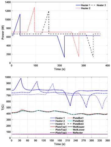
The resulting system Eq. (17) for the network model in Figure 1 was solved using the stiff ODE solver routine ODE45 in Matlab [31]. For fixed heat source values Qif, the system reached a steady state. Two sets of steady states were solved for, as shown below, with a time step of 0.1s. The choice of the time step here was based on the smallest time constant in the system, which is that of the heaters – of the order of ten seconds, as seen from Figure 2. Although the convergence to increases as the time step ® 0 [15, 32], for practical purposes, the time step could be chosen such that the model is able to accurately learn the highest frequency dynamics in the actual full order system.
Figure 2. (a) Evolution to steady state A (top) and (b) Evolution to steady state B (bottom)
The following steady states were used as initial conditions later for test cases:
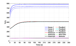
(1) Steady State (SSA) corresponds to QA f= [Q1f, Q2f, Q3f ] = [425W, 470W, 385W], and the evolution of the temperatures in the 12 nodes are shown in Figure 2a. The average wafer temperature was 266.5C. The three nodal temperatures were on the plate were Tp = [269.1, 266.1 264.4] C.
(2) Steady State (SSB) Corresponds to QB f = [625W, 710W, 665W], and the evolution of the temperatures in the 12 nodes are shown in Figure 2b. The average wafer temperature was 411.7C. The three nodal temperatures were on the plate were Tp = [415.3, 411.1, 408.8] C.
Several transient data sets generated from the model in Eq. (7) were used as training and test cases for the predictive models identified with modified and original DMDc. These data sets are described below.
4.1 Training data set
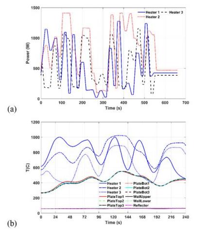
Typical interest in practical applications of heat transfer lie in heat-up, soak and cool down behavior of systems. Hence the training data of temperatures was generated using randomized ramp-up, dwell, and ramp-down signals as shown in Figure 3 starting from a baseline heat source corresponding to steady state A, Qf = QA f. The heat source magnitudes varied up to ±100% of the baseline values. The ramp-up-down durations varied between 10 to 16 s, and dwell time durations varied between 8 to 13s. The total duration of the signals was 660 s. The initial condition of the system was steady state A. The temperature variations for the 12 components are plotted in Figure 3. The plate temperatures varied between 178.6 and 551.6℃.
Figure 3. Training case: (a) Inputs (top) and (b) States (bottom)
4.2 Test data sets
Four sets of test data sets were used to compare with the DMDc model predictions. The test data sets were generated with the same time step of 0.1s. The simulations used either steady state A or B as the initial conditions of the components. The initial conditions, heat source input signals and the temperature evolutions for these sets are described below.
4.2.1 Square wave response
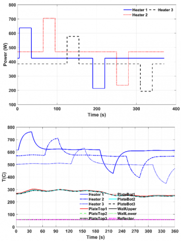
The input signal corresponded to ±50% square waves from the baseline values corresponding to states A and B. The inputs and outputs are depicted in Figure 4 and Figure 5, for initial conditions of states A & B.
Figure 4. Inputs and numerically solved states for square wave inputs, starting from steady state A
Figure 5. Inputs and numerically solved states for square wave input, starting from steady state B
4.2.2 Step response
The input signal at time=0 corresponded to a step function from the input heat source values corresponding to SSA, to those at SSB. The initial conditions were from SSA. The system allowed to evolve from SSA to SSB. The inputs are not shown in Figure 6 below since they are constant values after t=0.
Figure 6. Numerically solved states for step input, starting from steady state A and reaching state B
4.2.3 Ramp response
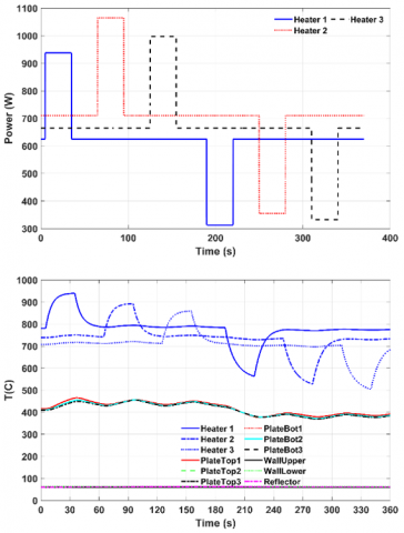
The input signal corresponded to ±50% sawtooth wave from the baseline values corresponding to B. The inputs and outputs are depicted in Figure 7, for initial conditions of states from B.
Figure 7. Inputs and numerically solved states for ramp input, starting from SSB
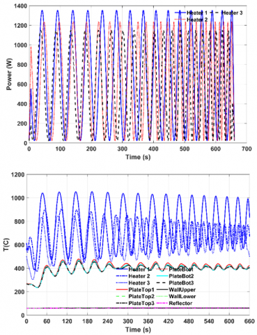
4.2.4 Chirp signal response
The input heat source values were from a chirp signal, with a frequency content varying from 0.02 to 0.033, 0.081, and 0.054Hz for heat sources 1, 2 and 3 respectively. The frequencies were selected approximately based on the below two criteria:
a) The ramp rates in each cycle were covered those in the training signal and higher or lower values, in order to test the validity of DMDc for conditions different from the training case.
b) The frequency values were specified so as to detect any input-output lag in the thermal behavior of the system in the reduced order model with sufficient accuracy, within the tested time range of 10 mins.
The mean value of the heat sources were such that the plate temperatures vary approximately around 400C, similar to the training signal. The initial condition was set using the steady state A. Results are shown in Figure 8.
Figure 8. Inputs and numerically solved states for chirp signal inputs, starting from SSA
The data from the numerical model was normalized in the following way, so that $0 \leq X_{i j} \leq 1$: X = (T-300)/1000, with Temperatures in degree Kelvins. The inputs (heat source values) were also normalized using 1000 W, so that the inputs are of the order of one. The scaling parameter’s value in Eq. (7) was fixed at 0.1. It was seen that increasing this to higher values (> 1) resulted in an instability in the system Eq. (10). The effect of the parameter on the accuracy of the ROM was negligible. This suggested that the added non-linearity (A2 term) was not contributing much to the accuracy of predictions.
5.1 Predictions using the identified models with DMDc
The models identified using the modified DMDc (Eq. 7-10) and the original DMDc method (Eq. 6-9) were used to predict the thermal evolution for different cases. The figures in the following sections show the comparison of modified DMDc predictions and the results from the original numerical model. Also, relative errors of predictions compared to the numerical simulation data are plotted and for the modified and the original DMDc methods.
Relative error was calculated using the L2 norm of the difference between the DMDc predictions and the numerical model’s results for the 12 nodes, divided by the L2 norm of the numerical model’s predictions. This error is plotted for all cases as a percentage.
Rel. Error $=\left\|X-X_{D M D}\right\|_{2} /\|X\|_{2}$ (18)
5.2 Results from training data sets
Figure 9. Predicted temperatures from modified DMDc for training set, compared with the original numerical results
The results from applying the modified DMDc to the training data set itself is shown in Figure 9. The errors are relatively within 5 to 10% for most of the time, except at 300s, when the relative errors are large, of the order of 25%, as shown in Figure 10. The high error in the predictions is possibly due to the high degree of non-linearity in the system, which is not captured completely by the linear operator in the DMDc. The introduction of the non-linear operator in the modified DMDc was not seen to decrease the magnitude of the error though. This could be due to the smaller magnitude of the non-linear operator compared to the linear operator in the modified DMDc method.
As mentioned in section 2.1, the dominant modes in the identified model were from the matrix A1. In the identified model using the training data, the resulting L2 norms were: ||A1|| = 7.62, and ||A2|| = 6.92e-6. The dominant contributor to the eigenmodes of the system, even considering the nonlinearity, were from the matrix A1. Thus, the identified system is only weekly non-linear. Nonetheless, the addition of the extra T4 terms helps to improve accuracy and stability depending on the choice of the multiplier s' in Eq. (7).
Figure 10. The relative prediction errors for the training case
5.3 Results from test data sets
Below the predicted results are compared with the numerical model’s data for different test cases. The relative errors are also computed and plotted for different test cases spanning input and initial condition variations.
5.3.1 Square wave response, at initial conditions SSA
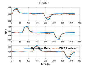
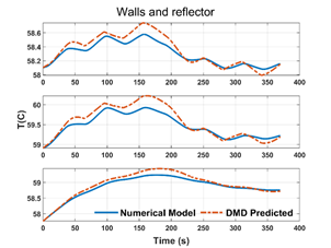
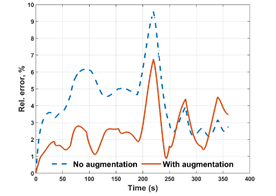
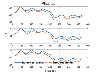
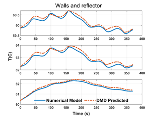
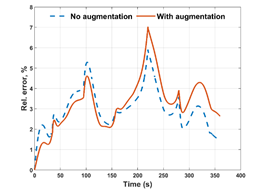
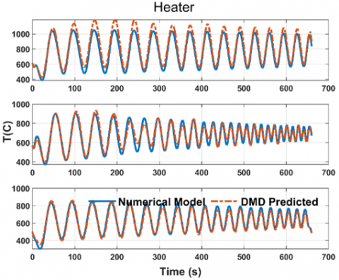
The predicted values from the identified model shows a decent correlation to the original data from the numerical model in Figure 11. The absolute deviation is within 80C, 10C and 0.3C for the heater, plate and the wall temperatures. The relative errors, plotted in Figure 12, is within 7% for the identified model using modified DMDc, and 10% with the DMDc method. The error is slightly lower with the modified DMDc model for most of the time duration.
5.3.2 Square wave response, at initial conditions SSB
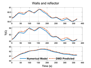
This case tests the identified model for an initial condition which is very different from the one in the training data. However, the values of the control input, that is, the heat source to the heaters were still within the range of those in the training data set. The values of the temperatures were also within the range of the temperature data in the training set. The absolute deviation increased for the plate temperatures to 25℃, whereas the deviations for the heater and walls were similar to the previous case, as shown in Figure 13.
The relative error for the DMDc identified model was lower compared to the modified DMDc method for most of the time duration. The difference in the relative errors of the two predictions was less than 1.2%, as seen in Figure 14.
Figure 11. Predicted temperatures from modified DMDc for square wave response, with initial condition SSA
Figure 12. Relative errors for square wave response, with initial condition SSA
Figure 13. Predicted temperatures from modified DMDc for square wave response, with initial condition SSB
Figure 14. Relative errors for square wave response, with initial condition SSB
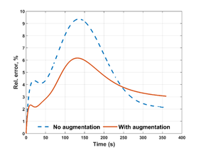
5.3.3 Step response, at initial conditions SSA
Figure 15. Predicted temperatures from modified DMDc for step response, with initial condition SSA
Figure 16. Relative errors for step response, with initial condition SSA
In this example, the system reaches steady state B starting from steady state A. The predictions showed a large deviation from the numerical simulation results for 100s < t < 150s, as shown in Figure 15. Even then, the relative errors were within 9% for the DMDc identified model and 6% for the modified DMDc identified model, seen in Figure 16.
5.3.4 Ramp input response, at initial conditions SSB
The predictions (Figure 17) were fairly similar to the numerical simulation values using both identifications in this case. The error magnitudes, in Figure 18, were within 1% of each other, although the errors from DMDc identification were smaller than those from the modified DMDc.
Figure 17. Predicted temperatures from modified DMDc for ramp input response, with initial condition SSB
Figure 18. Relative errors for ramp input response with initial condition SSB
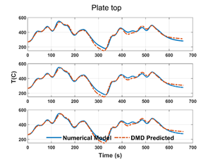
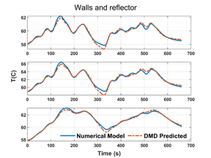
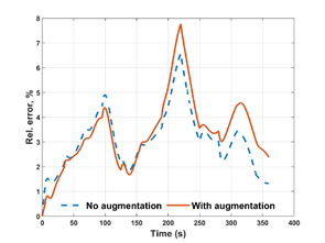
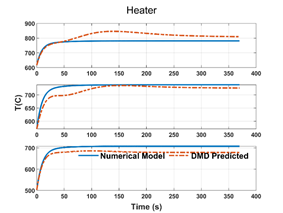
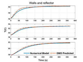
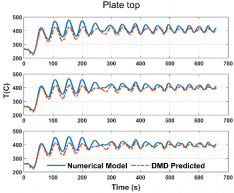
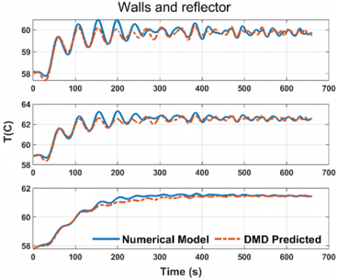
5.3.5 Chirp response, at initial conditions SSA
Figure 19. Predicted temperatures from modified DMDc for chirp input response, with initial condition SSA
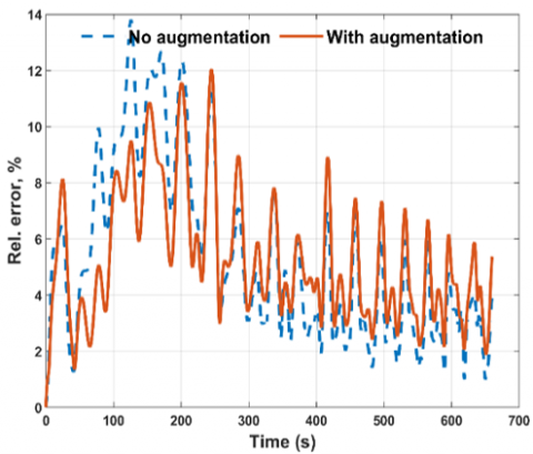
Figure 20. Relative errors for chirp input response with initial condition SSA
The chirp signal input contains frequency and ramp contents that are more different compared to the training signal in Figure 8. The response to the chirp signal was predicted well by both the DMDc identifications (Figure 19). The relative errors were slightly higher again near 100<t<150s time interval, as depicted in Figure 20. The relative errors were largely similar for both the identifications, although the peak error was lower using the modified DMDc identification.
The DMDc method has been used for non-solver intrusive model identification, order reduction and predictions. Although the problem considered here was simple and with small number of states (or components), the same method can be used for more complex systems with varying thermal properties, and with much larger number of states. Reasonably accurate and realistic predictions were obtained using the method. The original DMDc method was modified with constant and non-linear augmentation terms to improve the similarity of the identified system with the equations governing radiative heat transfer. The fourth order non-linear term can be used to position the eigenvalues for stability and the constant term provides for a better incorporation of time-independent boundary and volume conditions in the numerical model.
The identified models were tested with different initial conditions and actuation inputs, significantly different from the ones used to generate the training data. Even then, the identified models resulted in predictions within 10% relative error compared to the original numerical model. Augmenting the DMDc method improved the accuracy of predictions for the following cases - square wave input response, chirp input response and step response with the same model initial condition as training data. It did not improve the accuracy for other cases when the initial conditions were different, at SSB, from training data set. The non-linear augmentation term did not improve the accuracy of predictions, but changed the eigenvalues of the system slightly. However, the constant augmentation term did result in changes in predictions compared to the original DMDc method. When the number of boundary and volume conditions in the model are larger, the constant term in Eq. (7) is expected to further increase the accuracy of the predictions.
The use of more recent method of SINDYc could possibly provide a more precise system identification. However, uncertainties could exist in the convergence of the identification process itself, and the applicability to a fresh test data set. The DMDc method is simpler and provides a simple means to reduce the order of the system drastically, for systems with large number of states. The DMDc method also provides information on the dominant eigenvalues and the evolution of the dynamic modes of the system for a better understanding. Although the identified models in this study showed stable and reasonably accurate predictions for different conditions compared to the training data set, care should be taken in practical applications to test the identified models sufficiently for both accuracy and more importantly for stability, for different operating conditions and initial conditions of practical interest. In this article, the truthfulness of the derived models using DMDc with respect to only the numerical solution to the full set of theoretical governing equations has been addressed. The accuracy of the full order numerical model needs to be ensured with respect to the actual system using experiments, and calibration of the full order numerical model accordingly prior to practical applications.
|
x |
Generic state variable (any unit) |
|
u |
Input (W) |
|
n |
Number of states |
|
l |
Number of actuation inputs |
|
m |
Number of time steps |
|
q |
Truncated number of states |
|
r |
Radius (m) |
|
H,d |
Height, thickness (m) |
|
h |
Heat transfer coefficient (W/m2K) |
|
t |
Time (s) |
|
T |
Temperature (K) |
|
Q,s |
Heat source (W) |
|
K |
Conductivity (W/mK) |
|
D |
Distance between nodes (m) |
|
F |
View factor |
|
A |
Area (m2) |
|
k |
Thermal conductivity (W/mK) |
|
Greek symbols |
|
|
$\varepsilon$ |
Emissivity |
|
$\delta$ |
Kronecker delta |
|
$\sigma$ |
Steffan Boltzmann Constant, W/m2K |
|
Subscripts |
|
|
h |
Heater |
|
w |
Wall |
|
p |
Plate |
|
f |
Fluid |
|
A |
Steady State Condition A |
|
B |
Steady State Condtition B |
[1] Benner, P., Gugercin, S., Willcox, K. (2015). A survey of projection-based model reduction methods for parametric dynamical systems. SIAM Review, 57(4): 483-531. https://doi.org/10.1137/130932715
[2] Wang, Y., Song, H., Pant, K. (2014). A reduced-order model for whole-chip thermal analysis of microfluidic lab-on-a-chip systems. Microfluidics and Nanofluidics, 16(1-2): 369-380. https://doi.org/10.1007.s10404-013-1210-0
[3] Lin, Z., Xiao, D., Fang, F., Pain, C.C., Navon, I.M. (2017). Non‐intrusive reduced order modelling with least squares fitting on a sparse grid. International Journal for Numerical Methods in Fluids, 83(3): 291-306. https://doi.org/10.1002/fld.4268
[4] Kerschen, G., Golinval, J.C., Vakakis, A.F., Bergman, L.A. (2005). The method of proper orthogonal decomposition for dynamical characterization and order reduction of mechanical systems: An overview. Nonlinear Dynamics, 41(1): 147-169. https://doi.org/10.1007/s11071-005-2803-2
[5] Klie, H. (2013). Unlocking fast reservoir predictions via nonintrusive reduced-order models. In SPE Reservoir Simulation Symposium. Society of Petroleum Engineers. https://doi.org/10.2118/163584-MS
[6] Xiao, D., Lin, Z., Fang, F., Pain, C.C., Navon, I.M., Salinas, P., Muggeridge, A. (2017). Non‐intrusive reduced‐order modeling for multiphase porous media flows using Smolyak sparse grids. International Journal for Numerical Methods in Fluids, 83(2): 205-219. https://doi.org/10.1002/fld.4263
[7] Ogunmolu, O., Gu, X., Jiang, S., Gans, N. (2016). Nonlinear systems identification using deep dynamic neural networks. arXiv preprint arXiv:1610.01439.
[8] Sjöberg, J., Hjalmarsson, H., Ljung, L. (1994). Neural networks in system identification. IFAC Proceedings Volumes, 27(8): 359-382. https://doi.org/10.1016/S1474-6670(17)47737-8
[9] Kaiser, E., Kutz, J.N., Brunton, S.L. (2018). Sparse identification of nonlinear dynamics for model predictive control in the low-data limit. Proceedings of the Royal Society A, 474(2219): 20180335. https://doi.org/10.1098/rspa.2018.0335
[10] Brunton, S.L., Proctor, J.L., Kutz, J.N. (2016). Sparse identification of nonlinear dynamics with control (SINDYc). IFAC-PapersOnLine, 49(18): 710-715. https://doi.org/10.1016/j.ifacol.2016.10.249
[11] Schmid, P.J. (2010). Dynamic mode decomposition of numerical and experimental data. Journal of fluid mechanics, 656: 5-28. https://doi.org/10.1017/S0022112010001217
[12] Tu, J.H., Rowley, C.W., Luchtenburg, D.M., Brunton, S.L., Kutz, J.N. (2014). On dynamic mode decomposition: Theory and applications. Journal of Computational Dynamics, 1(2): 391-421. https://doi.org/10.3934/jcd.2014.1.391
[13] Chen, K.K., Tu, J.H., Rowley, C.W. (2012). Variants of dynamic mode decomposition: boundary condition, Koopman, and Fourier analyses. Journal of Nonlinear Science, 22(6): 887-915. https://doi.org/10.1007/s00332-012-9130-9
[14] Brunton, S.L., Proctor, J.L., Kutz, J.N. (2013). Compressive sampling and dynamic mode decomposition. arXiv preprint arXiv:1312.5186.
[15] Proctor, J.L., Brunton, S.L., Kutz, J.N. (2016). Dynamic mode decomposition with control. SIAM Journal on Applied Dynamical Systems, 15(1): 142-161. https://doi.org/10.1137/15M1013857
[16] Williams, M.O., Kevrekidis, I.G., Rowley, C.W. (2015). A data-driven approximation of the Koopman operator: Extending dynamic mode decomposition. Journal of Nonlinear Science, 8(1): 1-40. https://doi.org/10.1007/s00332-015-9258-5
[17] Benner, P., Himpe, C., Mitchell, T. (2018). On reduced input-output dynamic mode decomposition. Advances in Computational Mathematics, 44(6): 1751-1768. https://doi.org/10.1007/s10444-018-9592-x
[18] Kou, J., Zhang, W. (2019). Dynamic mode decomposition with exogenous input for data-driven modeling of unsteady flows. Physics of Fluids, 31(5): 057106. https://doi.org/10.1063/1.5093507
[19] Le Clainche, S., Vega, J.M. (2017). Higher order dynamic mode decomposition. SIAM Journal on Applied Dynamical Systems, 16(2): 882-925. https://doi.org/10.1137/15M1054924
[20] Jovanović, M.R., Schmid, P.J., Nichols, J.W. (2014). Sparsity-promoting dynamic mode decomposition. Physics of Fluids, 26(2): 024103. https://doi.org/10.1063/1.4863670
[21] Kutz, J.N., Fu, X., Brunton, S.L. (2016). Multiresolution dynamic mode decomposition. SIAM Journal on Applied Dynamical Systems, 15(2): 713-735. https://doi.org/10.1137/15M1023543
[22] Proctor, J.L., Brunton, S.L., Kutz, J.N. (2018). Generalizing Koopman theory to allow for inputs and control. SIAM Journal on Applied Dynamical Systems, 17(1): 909-930. https://doi.org/10.1137/16M1062296
[23] Bai, Z., Kaiser, E., Proctor, J. L., Kutz, J.N., Brunton, S.L. (2020). Dynamic mode decomposition for compressive system identification. AIAA Journal, 58(2): 561-574. https://doi.org/10.2514/1.J057870
[24] Ojo, S.O., Grivet-Talocia, S., Paggi, M. (2015). Model order reduction applied to heat conduction in photovoltaic modules. Composite Structures, 119: 477-486. https://doi.org/10.1016/j.compstruct.2014.09.008
[25] Botto, D., Zucca, S., Gola, M.M. (2007). Reduced-order models for the calculation of thermal transients of heat conduction/convection FE models. Journal of Thermal Stresses, 30(8): 819-839. https://doi.org/10.1080/01495730701415806
[26] Mathai, P.P. (2008). Application of reduced order modeling techniques to problems in heat conduction, isoelectric focusing and differential algebraic equations. PhD. Thesis, University of Maryland, Department of Aerospace Engineering, College Park, MD.
[27] Gartling, D.K., Hogan, R.E. (2010). Reduced Order Models for Thermal Analysis Final Report: LDRD Project No. 137807. (No. SAND2010-6352). Sandia National Laboratories. https://doi.org/10.2172/991534
[28] Wu, Z., Laurence, D., Utyuzhnikov, S., Afgan, I. (2019). Proper orthogonal decomposition and dynamic mode decomposition of jet in channel crossflow. Nuclear Engineering and Design, 344: 54-68. https://doi.org/10.1016/j.nucengdes.2019.01.015
[29] Howell, J.R., Siegel, R., Menguç, M.P. (2013). Thermal Radiation Heat Transfer (5th ed.). Boca Raton: Taylor and Francis.
[30] Howell, J.R. (2001). A Catalog of Radiation Heat Transfer Configuration Factors. University of Texas at Austin. http://www.thermalradiation.net/tablecon.html.
[31] Matlab. Version: 9.6.0.1072779 (R2019a). Natick, MA: The Mathworks Inc. https://www.mathworks.com/help/matlab/ref/ode45.html.
[32] Lu, H., Tartakovsky, D.M. (2020). Prediction accuracy of dynamic mode decomposition. SIAM Journal on Scientific Computing, 42(3): A1639-A1662. https://doi.org/10.1137/19M1259948