Xuejian Zhao
© 2021 IIETA. This article is published by IIETA and is licensed under the CC BY 4.0 license (http://creativecommons.org/licenses/by/4.0/).
OPEN ACCESS
If the crude oil in storage tank is directly heated without considering its temperature distribution, several problems will occur, namely, the thermal expansion of crude oil, and the uneven thickness of the condensate layer, bringing difficulty to the safe management of crude oil storage and transport. However, few scholars have analyzed the temperature field distribution of crude oil storage tank (COST) under heating, or the internal force of COST under static force. Thus, this paper probes into the thermal stress of tank wall, and the risk prevention and control of COST. Firstly, the heat transfer properties of COST were analyzed, an energy balance model was constructed for COST, and several variables were selected to evaluate the heat transfer effect of the tank under different heating modes, including thermal design power, temperature rise rate, and heat energy utilization rate. Next, the cross-section of COST wall was selected for thermal stress analysis. Based on the extremes of circumferential and vertical thermal stresses, the weak parts of COST susceptible to risks like leakage were determined, and several measures and suggestions were presented for reducing the risks of crude oil storage and transport.
crude oil storage tank (COST), thermal stress analysis, risk prevention and control, storage and transport
Currently, the storage and transport, and metering of crude oil do not pay much attention to the temperature change and stress state of the crude oil in storage tank [1-3]. The accurate metering of crude oil relies on the precision of temperature measurement [4-6]. According to the theories of heat transfer and thermodynamics, the inlet and outlet pipes and heating coils of crude oil storage tank (COST) all have an impact on the temperature field of the crude oil in the tank [7-10]. If the crude oil in storage tank is directly heated without considering its temperature distribution, several problems will occur, namely, the thermal expansion of crude oil, and the uneven thickness of the condensate layer, bringing difficulty to the safe management of crude oil storage and transport.
After long-term storage in COST, the crude oil will condensate as the temperature dropped to the right level [11-14]. Miansari et al. [15] designed a COST temperature detection and analysis system for real-time accurate monitoring of COST temperature, acquired real-time monitoring data on inlet/output temperature, horizontal/vertical temperature distribution in the tank, the horizontal temperature distribution on the outer wall, and the ambient temperature of the tank, and discussed the temperature distribution and temperature drop law in each part of the tank.
The tank capacity chart will have certain deviations, if the mean tank wall temperature is measured, ignoring the effect of changing temperature of the crude oil [16-19]. Hirokawa et al. [20] carried out Ansys Fluent simulation of an indoor tank model with different temperature rises and drops, compared the simulated and measured results at different positions, and verified the accuracy and effectiveness of their mathematical model for large COSTs. Kozłowska and Jadwiszczak [21] analyzed the distribution of crude oil flow field and temperature field in COST under tubular heating, oil loading/unloading heating, and hot oil circulation heating, measured the thermal design power and other indices of the tank through numerical discretization based on finite volume method, and effectively evaluated the flow and heat transfer properties of crude oil. Wang et al. [22] examined the thickness variation law of the thermal boundary layer beneath the roof of COST, and the composition of the vortex flows formed by the crude oil in the tank, under different heating modes. Cheng and Zhu [23] took the COST with thermal buoyancy jet features under oil loading/unloading as the object, and analyzed the change laws of crude oil temperatures at positions like the left and right sides of the jet trajectory, the tank top, the tank center, etc.
To rate the safety of COST, Miyazaki and Nakamura [24] constructed a multi-layer evaluation index system for storage tank risks, involving corrosion factors, equipment and facility factors, and other factors, and performed weight assignment and correction to these indices by a self-designed Bayesian feedback cloud model. Colombano et al. [25] introduced cloud reasoning, which simultaneously considers the stochasticity and fuzziness of storage tank risks, into the evaluation of COST risks, realized the conversion between qualitative indices and quantitative index values in storage tank integrity management, and objectively reflected the discreteness of index data. Targeting the heating and storage of waxy crude oil that is easy to condensate, highly viscous, and rheological, Mathew et al. [26] presented a mathematical model for the melting of waxy crude oil in waxy COST, explored the evolution laws of the temperature and flow fields under the effects of phase change between solid and liquid phases, and summarized the laws of heat transfer of crude oil and growth of condensate layer at different positions. Ono et al. [27] combined laminar flow model with large eddy simulation to calculate the increasing turbulence process of the crude oil in waxy COST, floating roof tank, and double-deck floating roof tank, and compared the melting of waxy crude oil layer with that of turbulence.
On the temperature field and stress field of COST, the existing research mainly tackles the improvement of thermal insulation performance during the construction phase, and the thermophysical properties of low-temperature crude oil. There is little report on the temperature field distribution COST under heating, or the internal force of COST under static force. Thus, this paper probes into the thermal stress and the risk prevention and control of COST. First of all, the heat transfer properties of COST were analyzed, an energy balance model was constructed for COST, and several variables were selected to evaluate the heat transfer effect of the tank under different heating modes, including thermal design power, temperature rise rate, and heat energy utilization rate. Next, the cross-section of COST wall was selected for thermal stress analysis. Finally, our algorithm was proved effective through experiments, and several measures and suggestions were presented for reducing the risks of crude oil storage and transport.
2.1 Construction of energy balance model
Figure 1. Simulation model for temperature field of COST
To ensure that the simulation of COST temperature field is sufficiently accurate for engineering applications, it is assumed that the space inside the tank is axially symmetric, the crude oil temperature is distributed evenly along the axis, the steel plates on the tank wall are of the same horizontal thickness, the foundation soil of the tank is a homogenous medium, and the heat radiation, internal heat source, and latent heat of condensation of crude oil are so small as to be negligible. Under these assumptions, a simulation model was created for the temperature field of COST (Figure 1). Based on the model, the three-dimensional (3D) heat transfer problem of COST can be transformed into a two-dimensional (2D) problem.
Let E1, EI, and E'I be the heat energy of the crude oil in the tank at time t1 relative to the reference temperature, the input heat energy, and the total energy after the input, respectively; E2, EO, and E'O be the heat energy of the crude oil in the tank at time t2 relative to the reference temperature, the output heat energy, and the total energy after the output, respectively; ES be the external heat supply to the tank; EL be the heat loss of the tank. Following the first law of thermodynamics, the energy balance relationship of the COST system can be described as:
$\left\{ \begin{matrix} {{{{E}'}}_{I}}+{{E}_{S}}={{E}_{L}}+{{{{E}'}}_{O}} \\ {{{{E}'}}_{I}}={{E}_{1}}+{{E}_{I}} \\ {{{{E}'}}_{O}}={{E}_{2}}+{{E}_{O}} \\\end{matrix} \right.$ (1)
2.2 Evaluation of heat transfer performance
The thermal design power, temperature rise rate, and heat energy utilization rate were selected to evaluate the heat transfer effect of the COST under different heating modes, and to examine their influence law on the heat transfer of the crude oil in the tank. The COST temperature measuring points were deployed as shown in Figure 2.
Figure 2. Distribution of temperature measuring points in COST
(1) Thermal design power
Firstly, the thermal design power of COST was defined and calculated to reveal the heat dissipation of the tank as the crude oil is being heated. Let L be the overall heat transfer coefficient of the tank; τb and τa be the mean temperature of crude oil in the tank and the temperature of the surrounding medium, respectively. Then, the thermal design power W of COST can be calculated by:
$W=L\left( {{\tau }_{b}}-{{\tau }_{a}} \right)$ (2)
Let LW, LD, and LB be the heat transfer coefficients of tank wall, tank roof, and tank bottom, respectively; SD, SW, and SB be the heat transfer areas of tank wall, tank roof, and tank bottom, respectively. Then, the overall heat transfer coefficient of the tank can be calculated by:
$L=\frac{{{L}_{W}}{{S}_{W}}+{{L}_{D}}{{S}_{D}}+{{L}_{B}}{{S}_{B}}}{{{S}_{W}}+{{S}_{D}}+{{S}_{B}}}$ (3)
Let η1W and η2W be the internal heat emission coefficient of the crude oil to the inner tank wall and that of the crude oil to the surrounding environment, respectively; η3W be the heat radiation coefficient of the outer tank wall to the surrounding environment; μW and μHP be the heat conductivities of tank wall and external insulation material, respectively; εW and εHP be the thicknesses of tank wall and external insulation material, respectively. Then, the overall heat transfer coefficient LW of COST wall can be calculated by:
${{L}_{W}}=\frac{1}{\frac{1}{{{\eta }_{1W}}}+\frac{{{\varepsilon }_{W}}}{{{\mu }_{W}}}+\frac{{{\varepsilon }_{HP}}}{{{\mu }_{HP}}}+\frac{1}{{{\eta }_{2W}}+{{\eta }_{3W}}}}$ (4)
Let εT-HP and μT-HP be the thickness and thermal conductivity of the tank roof insulation layer, respectively; εAL and μAL be the thickness and thermal conductivity of the air layer in the buoyancy chamber, respectively. For a vertical COST whose thermal resistance peaks in the insulation layer, the overall heat transfer coefficient LD of the tank roof can be calculated by:
${{L}_{D}}=\frac{1}{\frac{{{\varepsilon }_{T-HP}}}{{{\mu }_{T-HP}}}+\frac{{{\varepsilon }_{AL}}}{{{\mu }_{AL}}}}$ (5)
Let ηB be the heat emission coefficient from the crude oil to the tank bottom; εj and μj be the thickness and thermal conductivity of the j-th layer of sludge deposit and the bottom plate, respectively; RB be the radius of tank bottom; μS be the heat emission coefficient of the soil directly in contact with tank bottom. Then, the heat transfer coefficient LB of tank bottom can be calculated by:
${{L}_{B}}=\frac{1}{\frac{1}{{{\eta }_{B}}}+\sum{\frac{{{\varepsilon }_{j}}}{{{\mu }_{j}}}}+\frac{\pi {{R}_{B}}}{8{{\mu }_{S}}}}$ (6)
(2) Temperature rise rate
Secondly, the temperature rise rate of COST was defined and calculated to learn how the crude oil temperature in the tank changes under different heating modes. Let υH be the temperature rise rate of crude oil in COST during the heating process; Ψ1 and Ψ2 be the mean temperature of the crude oil in the tank at time t1 and t2, respectively; Δτ be the difference between Ψ1 and Ψ2. Then, the temperature rise rate of COST can be calculated by:
${{\upsilon }_{H}}=\frac{{{\Psi }_{2}}-{{\Psi }_{1}}}{\Delta \tau }$ (7)
(3) Heat energy utilization rate
Thirdly, the heat energy utilization rate of COST was defined and calculated to reveal the heat transfer law of the crude oil in the tank under different heating modes. The heat energy utilization rate υ of COST can be calculated by:
$\upsilon =\frac{{{{{E}'}}_{O}}}{{{E}_{S}}+{{{{E}'}}_{I}}}=\frac{{{E}_{2}}+{{E}_{O}}}{{{E}_{S}}+{{E}_{1}}+{{E}_{I}}}$ (8)
The EO and EI of tubular heating are both equal to zero. Let R be the tank diameter; Ψc be the reference temperature; ES be the heat energy supplied by the heating pipe to the crude oil in the tank from time t1 to time t2; Q1 and Q2 be the masses of the crude oil in the tank at t1 and t2, respectively; σ1 and σ2 be the specific heats of the crude oil in the tank at t1 and t2, respectively; Ψ1 and Ψ2 be the mean temperatures of the crude oil in the tank at t1 and t2, respectively; K1 and K2 be the liquid levels of the crude oil in the tank at t1 and t2, respectively. Then, formula (8) can be simplified as:
$\upsilon =\frac{{{E}_{2}}}{{{E}_{S}}+{{E}_{1}}}$ (9)
where,
$\left\{ \begin{matrix} {{E}_{S}}={{L}_{0}}rB\left( {{t}_{2}}-{{t}_{1}} \right) \\ {{E}_{1}}=\frac{\pi }{4}\rho {{R}^{2}}{{K}_{1}}{{\sigma }_{1}}\left( {{\Psi }_{2}}-{{\Psi }_{1}} \right) \\ {{E}_{2}}=\frac{\pi }{4}\rho {{R}^{2}}{{K}_{2}}{{\sigma }_{2}}\left( {{\Psi }_{2}}-{{\Psi }_{c}} \right) \\\end{matrix} \right.$ (10)
Let η1H and η2H be the internal heat emission coefficient from the steam to inner tank wall, and the external heat emission coefficient from the outmost layer of heating pipe to the crude oil, respectively; δj be the diameter of the j-th layer of sludge deposit on the inner wall of the pipe, considering the inner diameter of the pipe; δI and δO be the inner and outer diameters of the heating pipe, respectively. Then, the overall heat transfer coefficient LS of the steam from the heater to the crude oil in the tank satisfies:
${{L}_{S}}=\frac{1}{\left( \frac{1}{{{\eta }_{1H}}{{\delta }_{I}}}+\sum\limits_{j=1}^{M}{\frac{1}{2{{\mu }_{j}}}ln\frac{{{\delta }_{j+1}}}{{{\delta }_{j}}}}+\frac{1}{{{\eta }_{2}}{{\delta }_{M+1}}} \right){{\delta }_{O}}}$ (11)
Under turbulent flow, the η1H value can be derived from the heat emission of the forced movement of the crude oil in the storage tank:
$\text{Nu}=\frac{{{\eta }_{1H}}{{\delta }_{O}}}{\mu }=0.027R{{\text{e}}^{0.81}}\sqrt[3]{\Pr }$ (12)
where, Re is the Reynolds number that characterizes the ratio of dynamic viscosity to kinematic viscosity of the crude oil; Pr is the Prandtl number related to temperature. Let v be the flow velocity of crude oil; γ and σF be the kinematic viscosity and specific heat capacity of crude oil under qualitative temperature, respectively; μ and ρ be the thermal conductivity and density of fluid under qualitative temperature, respectively. Then, Re and Pr can be calculated by:
$R\text{e}=\frac{v{{\delta }_{O}}}{\gamma },\Pr =\frac{\gamma {{\sigma }_{F}}\rho }{\mu }$ (13)
Let RA be the additional thermal resistance. Ignoring the difference between 1/η1HδO, δO, and δOM+1, formula (11) can be simplified as:
${{L}_{S}}=\frac{1}{\frac{1}{{{\eta }_{2H}}}+{{R}_{A}}}$ (14)
Let μb be the thermal conductivity of crude oil under qualitative temperature; φ and M be two proportional coefficient and power exponent, respectively. Then, the value of η2H depends on the product between Pr value and the Grashof number Gr, which characterizes the buoyancy and viscous force in the convective heat transfer of natural fluids:
${{\eta }_{2}}=\varphi \frac{{{\mu }_{b}}}{{{\delta }_{O}}}{{\left( \text{Gr},\text{Pr} \right)}^{M}}$ (15)
Let a be the acceleration of gravity; α be the expansion coefficient of crude oil at qualitative temperature; Δτ' be the difference between mean temperature of crude oil and the temperature of exothermic tank wall. Then, the Gr value can be calculated by:
$\text{Gr}=\frac{a \alpha \Delta \tau {{\delta }_{O}}^{3}}{{{\gamma }^{2}}}$ (16)
Figure 3. COST model under oil loading/unloading heating mode
During oil loading/unloading, the cold oil in the tank exchanges heat with the hot oil entering the tank. As a result, the temperature of the crude oil in the tank gradually increases, while the liquid level remains the same. In this process, the temperature distribution of the crude oil in the tank might change, as heat is emitted from the unloaded oil and the tank wall to the environment. Figure 3 presents the COST model under oil loading/unloading heating mode.
Let ESR-I and ESR-O be the heat carried by the crude oil entering the tank via the inlet pipe and the heat carried by the crude oil leaving the tank via the outlet pipe, respectively; σSR-I, QSR-I, and ΨSR-I be the specific heat, mass, and temperature of the crude oil ejected by the oil pipe or nozzle, respectively; ΨSR-O be the temperature of the oil leaving the tank. Since the ESR-S equals zero under the oil loading/unloading heating mode, the heat energy utilization rate υSR of the tank under oil loading/unloading heating and hot oil circulation heating can be defined as:
${{\upsilon }_{SR}}=\frac{{{E}_{SR-2}}+{{E}_{SR-O}}}{{{E}_{SR-1}}+{{E}_{SR-I}}}$ (17)
where,
$\left\{ \begin{matrix} {{E}_{SR-I}}={{\sigma }_{SR-I}}{{Q}_{SR-I}}\left( {{\Psi }_{SR-I}}-{{\Psi }_{c}} \right) \\ {{E}_{SR-O}}={{\sigma }_{SR-O}}{{Q}_{SR-O}}\left( {{\Psi }_{SR-O}}-{{\Psi }_{c}} \right) \\\end{matrix} \right.$ (18)
The analysis results on the heat transfer process of COST indicate that the crude oil in the tank suffers from the thermal stress caused by the temperature gradient, even during the normal use of COST. The parts of the tank under relatively high thermal stress are susceptible to risks like leakage. If the low-temperature crude oil leaks, the temperature difference between the inside and outside of the tank will increase. The ensuing growth of thermal stress will definitely affect the performance of COST wall. Let h1 and h2 be the inner and outer radii of COST, respectively. Suppose the cylindrical tank has a fixed height. Then, the thermal stress of the axially symmetric COST can be calculated by:
$\left\{ \begin{matrix} {{\xi }_{h}}=\frac{\beta W}{1-\lambda }\left[ -\frac{1}{{{h}^{2}}}\int_{{{h}_{1}}}^{h}{\Delta \tau hdh+\frac{{{h}^{2}}-h_{i}^{2}}{{{h}^{2}}\left( h_{2}^{2}-h_{j}^{2} \right)}\int_{{{h}_{j}}}^{{{h}_{2}}}{\Delta \tau hdh}} \right] \\ {{\xi }_{\vartheta }}=\frac{\beta W}{1-\lambda }\left[ \frac{1}{{{h}^{2}}}\int_{{{h}_{1}}}^{h}{\Delta \tau hdh+\frac{{{h}^{2}}-h_{j}^{2}}{{{h}^{2}}\left( h_{2}^{2}-r_{j}^{2} \right)}\int_{{{h}_{j}}}^{{{h}_{2}}}{\Delta \tau hdh-\tau }} \right] \\ {{\xi }_{c}}=\frac{\beta W}{1-\lambda }\left[ \frac{2}{{{h}^{2}}\left( h_{^{2}}^{2}-h_{j}^{2} \right)}\int_{{{h}_{j}}}^{{{h}_{2}}}{\Delta \tau hdh-\Delta \tau } \right] \\\end{matrix} \right.$ (19)
The thermal stress problem on the cross-section of COST wall is a one-dimensional (1D) steady-state heat conduction problem. Let ∆τ1 and ∆τ2 be the temperature changes on the inner and outer surfaces of COST wall, respectively. Since ∆τ2=0, the 1D radial heat conduction can be described by the following differential equation:
$\frac{{{d}^{2}}\Delta \tau }{d{{h}^{2}}}+\frac{1}{h}\frac{d\Delta \tau }{dh}=0$ (20)
Solving Eq. (20):
$\Delta \tau =\Delta {{\tau }_{1}}ln\frac{{{h}_{2}}}{h}/\left( ln\frac{{{h}_{2}}}{{{h}_{1}}} \right)$ (21)
Formulas (21) and (19) can be combined to express thermal stress of 1D steady-state conduction:
$\left\{ \begin{matrix} {{\xi }_{h}}=\frac{\beta W\Delta {{\tau }_{1}}}{2\left( 1-\lambda \right)ln_{{{h}_{1}}}^{{{h}_{2}}}}\left[ -ln\frac{{{h}_{2}}}{h}-\frac{h_{1}^{2}}{h_{^{2}}^{2}-h_{1}^{2}}\left( 1-\frac{h_{2}^{2}}{{{h}^{2}}} \right)ln\frac{{{h}_{2}}}{{{h}_{1}}} \right] \\ {{\xi }_{\vartheta }}=\frac{\beta W\Delta {{\tau }_{1}}}{2\left( 1-\lambda \right)ln_{{{h}_{1}}}^{{{h}_{2}}}}\left[ 1-ln\frac{{{h}_{2}}}{h}-\frac{h_{1}^{2}}{h_{^{2}}^{2}-h_{1}^{2}}\left( 1-\frac{h_{2}^{2}}{{{h}^{2}}} \right)ln\frac{{{h}_{2}}}{{{h}_{1}}} \right] \\ {{\xi }_{c}}=\frac{\beta W\Delta {{\tau }_{1}}}{2\left( 1-\lambda \right)ln_{{{h}_{1}}}^{{{h}_{2}}}}\left( 1-ln\frac{{{h}_{2}}}{h}-\frac{h_{1}^{2}}{h_{^{2}}^{2}-h_{1}^{2}}ln\frac{{{h}_{2}}}{{{h}_{1}}} \right) \\\end{matrix} \right.$ (22)
Substituting h=hj and h=h2 into formula (22), the stresses on the inside and outside of COST tank can be obtained as:
$\left\{ \begin{matrix} {{\left( {{\xi }_{\vartheta }} \right)}_{h={{h}_{1}}}}={{\left( {{\xi }_{c}} \right)}_{h={{h}_{1}}}}=\frac{\beta W\Delta {{\tau }_{1}}}{2\left( 1-\lambda \right)ln_{{{h}_{1}}}^{{{h}_{2}}}}\left( 1-\frac{2h_{2}^{2}}{h_{2}^{2}-h_{1}^{2}}ln\frac{{{h}_{2}}}{{{h}_{1}}} \right) \\ {{\left( {{\xi }_{\vartheta }} \right)}_{h={{h}_{2}}}}={{\left( {{\xi }_{c}} \right)}_{h={{h}_{2}}}}=\frac{\beta W\Delta {{\tau }_{1}}}{2\left( 1-\lambda \right)ln_{{{h}_{1}}}^{{{h}_{2}}}}\left( 1-\frac{2h_{2}^{2}}{h_{^{2}}^{2}-h_{1}^{2}}ln\frac{{{h}_{2}}}{{{h}_{1}}} \right) \\\end{matrix} \right.$ (23)
By default, the outer radius of COST is much greater than the wall thickness. Then, formula (23) can be simplified as:
$\left\{ \begin{matrix} \frac{{{h}_{2}}}{{{h}_{1}}}=\frac{{{h}_{1}}+\left( {{h}_{2}}-{{h}_{1}} \right)}{{{h}_{1}}}=1+N \\ N=\frac{{{h}_{2}}-{{h}_{1}}}{{{h}_{1}}} \\\end{matrix} \right.$ (24)
The logarithms of h1 and h2 satisfy:
$ln\frac{{{h}_{2}}}{{{h}_{j}}}=N+\frac{{{N}^{2}}}{2}+\frac{{{N}^{3}}}{3}-...$ (25)
Substituting formulas (24) and (25) into formula (23):
$\left. \begin{align} & {{\left( {{\xi }_{\vartheta }} \right)}_{h={{h}_{1}}}}={{\left( {{\xi }_{c}} \right)}_{h={{h}_{1}}}}=\frac{\beta W\Delta {{\tau }_{1}}}{2\left( 1-\lambda \right)ln_{{{h}_{1}}}^{{{h}_{2}}}}\left[ 1+N \right] \\ & {{\left( {{\xi }_{\vartheta }} \right)}_{h={{h}_{2}}}}={{\left( {{\xi }_{c}} \right)}_{h={{h}_{2}}}}=\frac{\beta W\Delta {{\tau }_{1}}}{2\left( 1-\lambda \right)ln_{{{h}_{1}}}^{{{h}_{2}}}}\left( 1-\frac{N}{3} \right) \\ \end{align} \right\}$ (26)
By default, the inner radius of COST is much greater than wall thickness. Thus, N is so small as to be negligible. Then, formula (26) can be simplified as:
$\left.\begin{array}{l}\left(\xi_{\vartheta}\right)_{h=h_{1}}=\left(\xi_{c}\right)_{h=h_{1}}=\frac{\beta W \Delta \tau_{1}}{2(1-\lambda)} \\ \left(\xi_{\vartheta}\right)_{h=h_{2}}=\left(\xi_{c}\right)_{h=h_{2}}=\frac{\beta W \Delta \tau_{1}}{2(1-\lambda)}\end{array}\right\}$ (27)
If the low-temperature crude oil leaks and the variation ∆τ2 in outer surface temperature of COST wall does not equal zero, ∆τ1 can be replaced with the temperature difference between inner and outer surfaces, thereby solving the thermal stress. Formula (27) shows that the tensile stress and compressive stress are maximized at the same time on the inner and outer surfaces of COST wall.
Figure 4 presents the horizontal temperature changes of crude oil during heating and cooling processes, that is, how the temperature of the laminated crude oil in the COST changes. Within 20h, the crude oil temperature increased by 12.1℃, and decreased by 13.3℃, in the heating and cooling phases, respectively; in both phases, the crude oil on the tank roof was 1.5~2.8℃ hotter than that on the tank bottom. With the elapse of time, the crude oil temperature increased significantly in the heating phase, while that did not change obviously in the cooling phase; neither did the temperature of the crude oil in the middle and upper parts of the tank change significantly.
Figure 5 shows the horizontal viscosity-temperature curves of crude oils. The oil samples at the bottom of the light hole in Group A were more viscous and heavier than the Murban crude oil in Group B. The high viscosity is related to the sludge deposits at the tank bottom, namely, colloids and asphalts. Therefore, the crude oil at other positions had similar viscosity-temperature curves, except the highly viscous oil sample A-1 at the bottom of the light hole, and these curves could accurately reflect the viscosity of the crude oil in the tank.
Under windy and windless conditions, the crude oil was heated and cooled by 20h, respectively. The horizontal temperature of the crude oil in each situation was monitored. The monitoring results in Figure 6 show that the crude oil temperature under windy condition changed similarly as that under windless condition, during the heating process; the temperature rise rate maximized at 1.451℃/h under windless condition. Moreover, the crude oil temperature dropped faster under windy condition than under windless condition. The cooling rate peaked at 1.153℃/h in the presence of wind. Comparing the temperature curves in heating and cooling phases, it can be seen that the crude oil at different depths had a small temperature difference during the cooling phase, which gradually approached zero; during the heating phase, there was an obvious temperature gradient in the horizontal direction.
Figure 7 shows how the mean temperature of crude oil in COST changes with time, and Figure 8 compares the theoretical values of crude oil temperature in COST with the measured results. As shown in Figure 7, the mean temperature of crude oil lagged the ambient temperature, and both temperatures changed as sine curves with a certain periodicity. The comparison in Figure 8 shows that the calculated values had basically the same trend as the measured values. Without considering environmental disturbance, the error between the two sets of values was smaller than 3℃.
(a) Heating phase
(b) Cooling phase
Figure 4. Horizontal temperature changes of crude oil during heating and cooling processes
Figure 5. Horizontal viscosity-temperature curves of crude oils
Based on the change laws of crude oil temperature in COST reflected in Figures 7 and 8, the overall heat transfer coefficients of the COST were calculated for 2019-2020. Table 1 illustrates the relative changes of the mean temperature of crude oil and ambient temperature.
Based on the relationship between mean temperature of crude oil and ambient temperature (Table 1), the overall heat transfer coefficients of COST in each phase were calculated (Table 2).
The data in Tables 1 and 2 confirm that the ambient temperature mainly causes temperature rise and temperature drop to the crude oil in COST. In Table 2, the columns 1-2 and 6-9 correspond to the heating phase, where the crude oil is cooler than the environment; in this phase, the ambient temperature is transferred to the crude oil in COST via the tank wall, and the overall heat transfer coefficient fell between 0.8318W/m2·K and 0.3687W/m2·K. The columns 2-5 and 9-10 correspond to the cooling phase, where the crude oil is hotter than the environment; in this phase, the crude oil losses heat, and the overall heat transfer coefficient fell between 0.8124W/m2·K and 0.7519W/m2·K. These results verify that: during the heating phase, the crude oil has a low heat transfer rate, and the natural convection slows down; during the cooling phase, the crude oil has a fast heat transfer rate, and the natural convection picks up speed.
(a) 20h heating
(b) 20h cooling
Figure 6. Horizontal temperature curves of crude oil under windy and windless conditions
Figure 7. Crude oil temperature vs. ambient temperature
Figure 8. Measured crude oil temperature vs. calculated crude oil temperature
Table 1. Relative changes of the mean temperature of crude oil and ambient temperature
|
Start time |
End time |
Initial temperature of crude oil |
Final temperature of crude oil |
Initial ambient temperature |
Final ambient temperature |
Relationship |
|
19.1.15 |
19.3.15 |
19.7 |
9.3 |
2.4 |
9.3 |
Crude oil temperature $\geqq$ Ambient temperature |
|
19.3.15 |
19.9.15 |
9.2 |
12.5 |
9.6 |
12.1 |
Crude oil temperature $\leqq$ Ambient temperature |
|
19.9.15 |
20.2.5 |
12.6 |
-1.8 |
12.1 |
-2.7 |
Crude oil temperature $\geqq$ Ambient temperature |
|
20.2.5 |
20.5.25 |
-2.5 |
5.6 |
-2.5 |
5.4 |
Crude oil temperature $\leqq$ Ambient temperature |
|
20.5.25 |
20.7.30 |
5.1 |
-2.7 |
5.5 |
-2.9 |
Crude oil temperature $\geqq$ Ambient temperature |
|
20.7.30 |
20.12.10 |
-2.4 |
2.35 |
-2.3 |
23 |
Crude oil temperature $\leqq$ Ambient temperature |
Table 2. Overall heat transfer coefficients of COST in each phase
|
Serial number |
1 |
2 |
3 |
4 |
5 |
|
Start time |
19.1.5 |
19.2.24 |
19.4.2 |
19.6.05 |
19.7.15 |
|
End time |
19.2.24 |
19.3.20 |
19.5.30 |
19.7.15 |
19.9.2 |
|
Heat transfer coefficient |
0.7519 |
0.8215 |
0.7251 |
0.4357 |
0.3721 |
|
Serial number |
6 |
7 |
8 |
9 |
10 |
|
Start time |
19.12.5 |
20.2.6 |
20.4.22 |
20.7.21 |
20.9.5 |
|
End time |
20.2.6 |
20.3.15 |
20.5.31 |
20.8.25 |
20.10.9 |
|
Heat transfer coefficient |
0.3687 |
0.5321 |
0.8318 |
0.8124 |
0.8073 |
Table 3. Theoretical and simulated extremes of circumferential thermal stress of COST
|
Reference point |
No protection, no leakage |
No protection, leakage |
Protection, no leakage |
Protection, leakage |
||||
|
Inner wall |
Outer wall |
Inner wall |
Outer wall |
Inner wall |
Outer wall |
Inner wall |
Outer wall |
|
|
Theoretical result |
0.351 |
-0.363 |
28.512 |
-26.357 |
0.372 |
-0.365 |
2.158 |
-2.168 |
|
Simulated result |
0.365 |
-0.347 |
27.6 |
-27 |
-29 |
0.362 |
2.12 |
2.05 |
|
Error |
0.65% |
3.57% |
3.15% |
4.65% |
0.65% |
4.98% |
3.12% |
1.99% |
Figure 9. Crude oil temperature curves at different depths
The above analysis shows that the crude oil temperature in COST does not change significantly in the horizontal direction. To examine the vertical distribution law of the temperature field of the crude oil, the authors investigated how the crude oil temperature changes with ambient temperature at each depth. Figure 9 sums up the temperature field distribution of the crude oil at different depths below the COST roof (depth interval: 0.4m) in 2020. By comparing the curves in the figure with ambient temperature curve, it is possible to capture the changes of crude oil temperature with ambient temperate at different depths. It can be inferred that the temperature of the crude oil in COST changed cyclically with the ambient temperature in most time; the only exception lies in the loading/unloading period, where the crude oil temperature changed significantly.
To verify its effectiveness, the proposed calculation method for the thermal stress on the cross-section of COST wall was applied to compute the extremes of circumferential and vertical thermal stresses with and without 1,2,3-Trichloropropane (TCP) protection, and in the absence/presence of crude oil leakage. The theoretical results are compared with simulated results in Tables 3 and 4. As shown in Table 3, the theoretical and simulated values for circumferential component of thermal stress differed by less than 5%, meeting the precision accuracy. The small error is resulted from the simplification of the calculation formula and the difference between boundary conditions and actual situation. As shown in Table 4, the theoretical and simulated values for vertical component of thermal stress differed by less than 10%, indicating that the two sets of values agree well with each other. In the absence of crude oil leakage, the error between the two sets of values fell in 8-10%, within the controllable range. Hence, our calculation method can effectively reflect the risk degree of COST.
Table 4. Theoretical and simulated extremes of vertical thermal stress of COST
|
Reference point |
No protection, no leakage |
No protection, leakage |
Protection, no leakage |
Protection, leakage |
||||
|
|
Inner wall |
Outer wall |
Inner wall |
Outer wall |
Inner wall |
Outer wall |
Inner wall |
Outer wall |
|
Theoretical result |
0.361 |
-0.375 |
27.825 |
-28.567 |
0.362 |
-0.331 |
2.732 |
-2.139 |
|
Simulated result |
0.357 |
-0.347 |
28.7 |
-26.7 |
0.371 |
0.317 |
2.37 |
2.32 |
|
Error |
8.3% |
9.3% |
0.003% |
0.23% |
8.2% |
9.7% |
0.02% |
2.98% |
(a) Gravity effect
(b) Water pressure effect
(c) Prestress effect
(d) Hydraulic effect
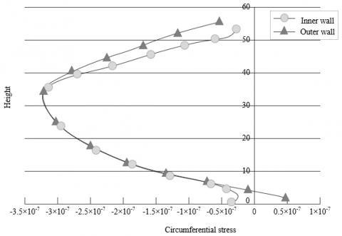
Figure 10. Circumferential thermal stresses of COST wall under different loads
Figure 10 shows the circumferential thermal stress curves of COST wall under four different loads. It can be observed that, under the four loads of gravity, water pressure, prestress, and hydraulic force, there was no great difference between the trends of circumferential thermal stress on the inner and outer walls of COST. Overall, the circumferential thermal stress peaked at 1/3 and 2/3 of tank heights. The thermal stress was relatively small on the outer wall near the center of the tank, and relatively large on the inner wall near the two ends. This proves that the direction of unfavorable load control changes with the height. To improve the safety and reduce the risk of COST storage and transport, the parts of the tank wall under relatively high thermal stress should be reinforced during the design phase, and measures should be taken to prevent crude oil from leaking.
This paper analyzes the thermal stress of COST and discusses how to prevent and control the risks of crude oil storage and transport. Firstly, the heat transfer features of COST were analyzed, and an energy balance model was built for COST. On this basis, COST thermal design power, temperature rise rate, and heat energy utilization rate were selected as the variables to evaluate the heat transfer effect of the tank under different heating modes. After that, the thermal stress on the cross-section of COST wall was calculated in details. Then, the horizontal temperature changes of the crude oil were tested under windy and windless conditions, and the measured temperatures were compared with the calculated values. The authors also analyzed the variation in crude oil temperature at different depths, calculated the extremes of circumferential and vertical heat stresses with and without TCP protection, in the presence/absence of crude oil leakage, and identified the weak parts of COST that are susceptible to risks like leakage. Finally, several measures and suggestions were given to reduce the risks of crude oil storage and transport.
[1] Sassine, N., Donzé, F.V., Harthong, B., Bruch, A. (2018). Thermal stress numerical study in granular packed bed storage tank. Granular Matter, 20(3): 1-15. https://doi.org/10.1007/s10035-018-0817-y
[2] Ismaeel, H.H., Yumrutaş, R. (2020). Thermal performance of a solar‐assisted heat pump drying system with thermal energy storage tank and heat recovery unit. International Journal of Energy Research, 44(5): 3426-3445. https://doi.org/10.1002/er.4966
[3] Jha, V.K., Banerjee, K., Bhaumik, S.K. (2021). Enhanced thermal stability of novel helical-finned jacketed stirred tank heater. Applied Thermal Engineering, 184: 116250. https://doi.org/10.1016/j.applthermaleng.2020.116250
[4] Khurana, H., Tiwari, S., Majumdar, R., Saha, S.K. (2021). Comparative evaluation of circular truncated-cone and paraboloid shapes for thermal energy storage tank based on thermal stratification performance. Journal of Energy Storage, 34: 102191. https://doi.org/10.1016/j.est.2020.102191
[5] Jadhav, I.B., Bose, M., Bandyopadhyay, S. (2020). Optimization of solar thermal systems with a thermocline storage tank. Clean Technologies and Environmental Policy, 22(5): 1069-1084. https://doi.org/10.1007/s10098-020-01849-4
[6] Riahi, S., Liu, M., Jacob, R., Belusko, M., Bruno, F. (2020). Assessment of exergy delivery of thermal energy storage systems for CSP plants: Cascade PCMs, graphite-PCMs and two-tank sensible heat storage systems. Sustainable Energy Technologies and Assessments, 42: 100823. https://doi.org/10.1016/j.seta.2020.100823
[7] Berdnikov, V.S., Mitin, K.A. (2020). Influence of thermal conductivity of the partition wall on non-stationary conjugate natural convective heat exchange and temperature fields in the walls of a rectangular fuel tank. In Journal of Physics: Conference Series, IOP Publishing, 1677(1): 012180. https://doi.org/10.1088/1742-6596/1677/1/012180
[8] Kim, M.H., Lee, Y.T., Gim, J., Awasthi, A., Chung, J.D. (2019). New effective thermal conductivity model for the analysis of whole thermal storage tank. International Journal of Heat and Mass Transfer, 131: 1109-1116. https://doi.org/10.1016/j.ijheatmasstransfer.2018.11.122
[9] Li, Y., Huang, G., Xu, T., Liu, X., Wu, H. (2018). Optimal design of PCM thermal storage tank and its application for winter available open-air swimming pool. Applied Energy, 209: 224-235. https://doi.org/10.1016/j.apenergy.2017.10.095
[10] Baissi, M.T., Touafek, K., Khanniche, R., Boutina, L., Khelifa, A. (2018). Numerical analysis of baffles effect on thermal storage capacity inside hot water storage tank. In 2018 6th International Renewable and Sustainable Energy Conference (IRSEC) IEEE, pp. 1-5. https://doi.org/10.1109/IRSEC.2018.8702907
[11] Elfeky, K.E., Ahmed, N., Naqvi, S.M.A., Wang, Q. (2019). Numerical investigation of the melting temperature effect on the performance of thermocline thermal energy storage tank for CSP. Energy Procedia, 158: 4715-4720. https://doi.org/10.1016/j.egypro.2019.01.731
[12] Espinosa, S.N., Jaca, R.C., Godoy, L.A. (2019). Thermal effects of fire on a nearby fuel storage tank. Journal of Loss Prevention in the Process Industries, 62: 103990. https://doi.org/10.1016/j.jlp.2019.103990
[13] Zhai, X.M., Wang, H. (2016). Influence factors of thermal stress in the construction period of the concrete outer tank for 160 000 m3 LNG storage. Harbin Gongye Daxue Xuebao/Journal of Harbin Institute of Technology, 48(6): 92-97. https://doi.org/10.11918/j.issn.0367-6234.2016.06.015
[14] Rodrigues, F.A., de Lemos, M.J. (2020). Effect of porous material properties on thermal efficiencies of a thermocline storage tank. Applied Thermal Engineering, 173: 115194. https://doi.org/10.1016/j.applthermaleng.2020.115194
[15] Miansari, M., Nazari, M., Toghraie, D., Akbari, O.A. (2020). Investigating the thermal energy storage inside a double-wall tank utilizing phase-change materials (PCMs). Journal of Thermal Analysis and Calorimetry, 139(3): 2283-2294. https://doi.org/10.1007/s10973-019-08573-2
[16] Kumar, B., Abhishek, A., Chung, J.D. (2020). New effective thermal conductivity model for the analysis of unconstrained melting in an entire thermal storage tank. Journal of Energy Storage, 30: 101447. https://doi.org/10.1016/j.est.2020.101447
[17] Cheng, X., Sun, L., Ma, H., Han, M., Zhang, R. (2015). Thermal stress and crack distribution of concrete dome of spherical LNG storage tank. Journal of China University of Petroleum, 39(5): 130-136. https://doi.org/10.3969/j.issn.1673-5005.2015.05.018
[18] Zhu, X., Cheng, X., Peng, W., Zi, G. (2014). Stress distribution and fracture pattern analysis of spherical LNG storage tank dome caused by thermal load. Shiyou Xuebao/Acta Petrolei Sinica, 35(5): 993-1000. https://doi.org/10.7623/syxb201405022
[19] Cheng, X.D., Han, M.Y., Peng, W.S., Zhu, X.J., Li, J.L. (2014). Thermal stress and crack distribution of the concrete outside of an LNG storage tank during construction. Natural Gas Industry, 34(9): 107-112. https://doi.org/10.3787/j.issn.1000-0976.2014.09.017
[20] Hirokawa, Y., Nishi, H., Yamada, M., Zama, S., Hatayama, K. (2012). Study on damage of a floating roof-type oil storage tank due to thermal stress. In Applied Mechanics and Materials. Trans Tech Publications Ltd, 232: 803-807. https://doi.org/10.4028/www.scientific.net/AMM.232.803
[21] Kozłowska, K., Jadwiszczak, P. (2018). The impact of inflow velocity on thermal stratification in a water storage tank. In E3S Web of Conferences. EDP Sciences, 44: 00079. https://doi.org/10.1051/e3sconf/20184400079
[22] Wang, K., Satyro, M.A., Taylor, R., Hopke, P.K. (2018). Thermal energy storage tank sizing for biomass boiler heating systems using process dynamic simulation. Energy and Buildings, 175: 199-207. https://doi.org/10.1016/j.enbuild.2018.07.023
[23] Cheng, X.D., Zhu, X.J. (2012). Thermal stress analysis on external wall of LNG storage tank and the design of pre-stressed reinforcement. Acta Petrolei Sinica, 33(3): 499-505. https://doi.org/10.7623/syxb201203024
[24] Miyazaki, K., Nakamura, S.A. (2004). Study on numerical analysis of cracks in PC LNG storage tank foundation slab caused by thermal stress. Ishikawajima Harima Engineering Review, 44(2): 91-99.
[25] Colombano, S., Davarzani, H., van Hullebusch, E.D., Huguenot, D., Guyonnet, D., Deparis, J., Ignatiadis, I. (2021). Comparison of thermal and chemical enhanced recovery of DNAPL in saturated porous media: 2D tank pumping experiments and two-phase flow modelling. Science of The Total Environment, 760: 143958. https://doi.org/10.1016/j.scitotenv.2020.143958
[26] Mathew, A., Nadim, N., Chandratilleke, T.T., Humphries, T.D., Paskevicius, M., Buckley, C.E. (2021). Performance analysis of a high-temperature magnesium hydride reactor tank with a helical coil heat exchanger for thermal storage. International Journal of Hydrogen Energy, 46(1): 1038-1055. https://doi.org/10.1016/j.ijhydene.2020.09.191
[27] Ono, H., Ohtani, Y., Matsuo, M., Yamaguchi, T., Yokoyama, R. (2021). Optimal operation of heat source and air conditioning system with thermal storage tank using nonlinear programming. Energy, 222: 119936. https://doi.org/10.1016/j.energy.2021.119936