Samira Noui* | Saadi Bougoul | Yassine Demagh
© 2021 IIETA. This article is published by IIETA and is licensed under the CC BY 4.0 license (http://creativecommons.org/licenses/by/4.0/).
OPEN ACCESS
Closed greenhouse systems optimize internal climatic conditions for both reducing energy loss and high-quality yields. Nevertheless, careful monitoring of the parameters of the microclimate requires a better understanding of the thermal phenomena that coexist at the same time inside the greenhouses. In the present study, the surface radiation effect on the natural convection in the greenhouse was investigated numerically based a turbulent unsteady model. The k-ε model was adopted for the turbulent flow and the discrete ordinate (DO) method for the radiation heat transfer. Assuming a no isotherm conditions at the floor and roof faces of the greenhouse and for a Rayleigh number ranges from 0.6×10¹⁰ to 2.3×10¹⁰. The results showed a strong radiation effect on the thermal behavior near the walls and considerably reduces the flow dynamics within the greenhouse. The contribution of the radiation heat transfer on the total Nusselt number at least 50% greater than that without. The results obtained for the selected values of Rayleigh numbers are in good agreement with the experimental data of the literature.
greenhouse, natural convection, numerical simulation, radiation heat transfer, turbulence
Greenhouses are high and sustainable crop production systems that protect the plants from external conditions, which are sometimes unfavourable. They are in continuous interaction with the external climatic conditions imposed on it. The knowledge of these conditions, the geometric and the physical properties of these systems should allow determining the instantaneous variation of the microclimate inside it. A greenhouse is usually composed of four different parts: the soil, the plant, the indoor air and the walls separating the inside from the outside. In this system many physical and biological mechanisms occur, governed by the exchanges of mass, heat and momentum transfers [1]. The various modes of heat exchange must be well identified and known inside the greenhouse and its components [2]. The originality of the greenhouse is in its property of transmitting a large part of the solar radiation, between 400 and 700 nm, which greatly contributes to the process of photosynthesis. This is why short wavelength radiation heat exchanges have been the subject of very close attention [3, 4]. All these works constitute a fairly complete reference to predict the transmission of the solar radiation within greenhouses. Besides, radiation heat exchanges of long wavelength occur between the solid components of the greenhouse (soil, plant and walls) and the outside environment. Due to their infrared transmission properties and their materiel nature, covers are the most important elements in these exchanges that characterize the amount of intercepted radiation and have been widely studied by Nijskens et al. [5-7]. While the experimental studies are difficult to achieve, numerical simulations provide a powerful tool for the computing, in time and in space, various physical parameters. Several Computational Fluid Dynamics (CFD) studies related to the radiation heat transfer have been carried out [8-10].) and just to name a few). The thermal boundary conditions set by these authors were: A constant temperature deduced from the measurements made in-situ, or a heat flux deduced indirectly from the energy balances taking into account effects of the radiation heat transfer.
Microclimate studies in greenhouses were also conducted by solving the radiation heat transfer equation coupled with the equation of energy [11, 12]. The Discrete Ordinates (DO) model was used to solve the RTE for both long and shortwave [13, 14]. Other authors have studied the effect of external climatic conditions on the microclimate inside the greenhouse [15-18], their results provide very precise indications of the management of the greenhouse system.
Alternatively [19-22], present numerical results to predict the mass transfer of the vapor between the crop and the inside air of the greenhouse.
The radiation exchanges between the different elements of the greenhouse have stimulated great interest due to their importance in basic by many authors. This study allows completing the research works done by the numerical simulation of the radiation heat transfer using DO radiation model. The aim of this work is to highlight the effects of the surface radiation on the heat transfer balance and the airflow dynamics inside the greenhouse, which will allow understanding in more details the physical phenomenon that governs the microclimate inside this system and consequently lead to a good management of the greenhouse microclimate.
2.1 Governing equations
The studied flow is described by the general transport equation shown below, where the variables velocity and the associated temperature T can be determined from the conservation equations of mass, momentum and energy. The transport equation for unsteady and two-dimensional flow is given by:
$\frac{\partial \phi}{\partial t}+\frac{\partial}{\partial x_{j}}\left(u_{j} \phi\right)=\frac{\partial}{\partial x_{j}}\left(\Gamma_{\phi} \frac{\partial \phi}{\partial x_{j}}\right)+S_{\phi}$ (1)
where, $\phi$ is the transport variable. $u_{j}$: The velocity component, $\Gamma_{\varphi}$: The diffusion coefficient and $S_{\phi}$: the source term. To take into account of the buoyancy forces, the Boussinesq approximation has been applied to the studied geometry. The k-e model was adopted that led to two supplementary equations for the turbulent energy k and its dissipation rate ε. The choice of this model resulted from some of the important numerical studies on turbulent natural convection [23-25]. These numerical studies demonstrate the capabilities of various turbulence models to predict turbulent natural convective flow in enclosures. The different transport equations are shown in the Table 1 and further details can be found in the refs. [26, 27].
Table 1. Transport equations
|
Equation |
Mathematical form |
|
Continuity equation |
$\frac{\partial \rho}{\partial t}+\frac{\partial\left(\rho u_{i}\right)}{\partial x_{i}}=0$ |
|
Momentum equation |
$\frac{\partial\left(\rho u_{i}\right)}{\partial t}+\frac{\partial\left(\rho u_{j} u_{i}\right)}{\partial x_{j}}=-\frac{\partial P}{\partial x_{i}}+$$\frac{\partial}{\partial x_{i}}\left(\mu \frac{\partial u_{i}}{\partial x_{j}}-\rho \overline{u_{l}^{\prime} u_{j}^{\prime}}\right)-\rho \beta\left(T-T_{0}\right) g_{i}$ |
|
Kinetic energy equation |
$\frac{\partial(\rho k)}{\partial t}+\frac{\partial\left(\rho u_{i} k\right)}{\partial x_{i}}=\frac{\partial}{\partial x_{i}}\left[\left(\mu+\frac{\mu_{t}}{\sigma_{k}}\right) \frac{\partial k}{\partial x_{i}}\right]+$$P_{k}+G_{k}-\rho \varepsilon$ |
|
Dissipation of turbulent kinetic energy equation |
$\frac{\partial(\rho \varepsilon)}{\partial t}+\frac{\partial\left(\rho u_{i} \varepsilon\right)}{\partial x_{i}}=\frac{\partial}{\partial x_{i}}\left[\left(\mu+\frac{\mu_{t}}{\sigma_{\varepsilon}}\right) \frac{\partial \varepsilon}{\partial x_{i}}\right]+$$\frac{\varepsilon}{k}[\underbrace{C_{\varepsilon 1}\left(P_{k}+C_{\varepsilon 3} G_{k}\right.})-\underbrace{C_{\varepsilon 2} \rho \varepsilon}]$ |
|
Energy equation |
$\frac{\partial(\rho T)}{\partial t}+\frac{\partial\left(\rho u_{i} T\right)}{\partial x_{i}}=\frac{\partial}{\partial x_{i}}\left(\frac{\lambda}{C_{p}} \frac{\partial T}{\partial x_{i}}-\right.$$\left.\overline{\rho u_{j}^{\prime} T^{\prime}}\right)+\frac{S_{r}}{C_{p}}$ |
The radiation heat transfers are introduced into the energy equation via the source term Sr, it is defined as:
$S_{r}=-\operatorname{div}\left(q_{r}\right)$ (2)
$S_{r}$ is computed once the spatial and directional fields of the luminance are known throughout the computational domain, which requires the resolution of the radiation transfer equation [28]. Radiation heat transfers are assumed by introducing the discrete ordinates model (DO). This model transforms the integro-differential equation of heat transfer into a set of simultaneous algebraic equations by replacing the directional variation of the radiation intensity with a discrete set of ordinates [29]. Thus,
$\nabla[I(\vec{r}, \vec{s}) \cdot \vec{s}]+\left(a+\sigma_{s}\right) \cdot I(\vec{r}, \vec{s})$$=a \cdot n^{2} \frac{\sigma T^{4}}{\pi}+\frac{\sigma_{s}}{4 \pi} \int_{0}^{4 \pi} I\left(\vec{r}, \vec{s}^{\prime}\right) \Phi\left(\vec{s}^{\prime}, \vec{s}\right) d \Omega$ (3)
where, $\vec{r}$: is the position vector, $\vec{s}$: is the direction vector, $\overrightarrow{s^{\prime}}$: is the distribution vector of direction, $a$: is the absorption coefficient, $n$: is the refractive index, $\sigma_{s}$: is the scattering coefficient, $I$: is the radiation intensity which depends of the position $\vec{r}$ and the direction $\vec{s}$, $T$: is the local temperature, $\Phi$: is the phase function and $\Omega$: is the solid angle.
It is found that the surface radiation does not modify the governing equations of movement $\left(a=0, \sigma_{s}=0\right)$ but only affects the thermal boundary conditions. The natural convection-surface radiation coupling is done through the thermal boundary conditions.
The model assumes that the radiation heat transfer is mainly done by the walls. For a surface behaving like a gray body, the incident radiative heat flux at the wall being;
${{q}_{in}}=\int_{\vec{s},\vec{n}>0}{{{I}_{incident}}}\vec{s}\cdot \vec{n}d\Omega $ (4)
The net radiative flux leaving the surface being:
${{q}_{out}}=\left( 1-{{\varepsilon }_{r}} \right){{q}_{in}}+{{n}^{2}}{{\varepsilon }_{r}}\sigma T_{8}^{4}$ (5)
where, n; is the refractive index of the medium next to the wall n=1.
2.2 Geometry and boundary conditions
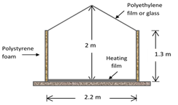
The reduced scale of the studied configuration of the greenhouse is showed in Figure 1. It has the dimensions: 2.2 m long, 2 m high and 1.5 m wide, the greenhouse is supplied with a commercial heating film on the floor. The roof is made of polyethylene film or glass of 3 mm thick and the adiabatic side walls are constituted by panels of 5 cm of expanded polystyrene. The choice of such a configuration is dictated by the existence of the experimental data of the paper [30], which was used for comparison. The energy balance at the roof can be written as:
${{q}_{mixed}}={{h}_{ext}}\left( T-{{T}_{ext}} \right)+{{\varepsilon }_{ext}}\sigma \left( {{T}^{4}}-T_{sky}^{4} \right)$ (6)
The first term in the right hand side represents the convective heat flux to the outside and the second term represents the radiation heat flux to the sky. The temperature of the sky being [31]:
${{T}_{sky}}=0.0559~T_{ext}^{1.5}$ (7)
The outside temperature [30] and external heat transfer coefficient [32] are defined by:
$\left\{ \begin{array}{*{35}{l}} {{T}_{ext}}=292.4K \\ {{h}_{ext}}=0.95+6.76{{V}^{0.49}} \\ \text{ where: }{{T}_{roof}}>{{T}_{ext}}\text{and }V\le 6.3{}^{m}/{}_{s} \\\end{array} \right.$ (8)
To reproduce the incoming solar radiation, as absorbed by the floor, Lamrani et al. [30] used an electrically heated film which releases adjustable heat flux densities.
In this study, the radiation heat transfers between the inner walls of the greenhouses were accounted for. The walls are assumed to be grey, diffuse and opaque. In order to evaluate the maximum effect of the radiation exchange on the airflow and heat transfer, the walls are assumed as blackbody (ε=1). The air (Pr=0.71) was supposed transparent non-participating medium.
Figure 1. The greenhouse configuration [30]
2.3 Grid independence tests and validation of the numerical model
The governing equations including the two additional transport equations for the turbulence kinetic energy (k) and the turbulence dissipation rate (e) with the specified boundary and initial conditions are solved using the CFD code Fluent 6.3. With reference to [27], during the meshing process, more nodes are placed inside the viscous sub-layer to capture the high resolution of gradients near the wall region and to ensure the satisfaction of the requirement $\left(y^{+}=y u_{\tau} / v<1\right)$ at the first grid point close to the wall, where $u_{z}$ is the frictional velocity given by $\sqrt{\tau_{w} / \rho}$ and $\tau_{w}$ being the wall shear stress.
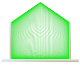
The numerical solution of the governing differential equations is obtained by using a finite volume technique and the resulting equations are iteratively solved. The physical model is generated using the pre-processing software Gambit (Version 2.3) as shown in Figure 2. It was meshed using quadratic elements no-uniformly distributed. An implicit scheme with second-order accuracy is adopted to match the solution. To discrete the governing equations, the PRESTO scheme is utilized for the pressure term whereas the Second Order Upwind scheme is adopted for the others. The SIMPLE algorithm is used for solving the pressure-velocity linked equation.
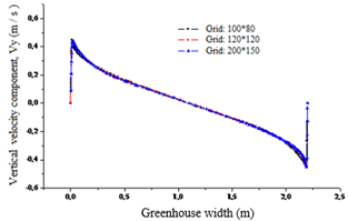
Since the solution should be independent of grids, the grid independence tests have been made for a Rayleigh number of $2.3 \times 10^{10}$. Three different grid structures are investigated $100 \times 80,120 \times 120$ and $200 \times 150$ cells. Figure 3 shows the trend of the vertical mean velocity component at the mid- height of the greenhouse.
Figure 2. Meshing of the studied configuration
Figure 3. Grid independence tests
The dynamics field was not affected by the refinement. While the maximum relative error of the average Nusselt number is less than 0.2% from these results.
To validate the mathematical model, comparisons between the numerical results and the experimental correlation by Lamrani et al. [30]. are provided varying the heat flux densities at the floor, which led to various Rayleigh numbers (Ra) as summarised in Table 2. Uniform grids have been used with logarithmic wall functions for the numerical simulations and the experimental correlation by the paper [30], in form of the surface heat transfer coefficient between soil surface and air in greenhouse being,
$h=5.2\left(T_{S}-T_{a}\right)^{0.33}$ (9)
The results and relative errors are also reported in Table 2 and showed an excellent agreement, with a maximum deviation of 4.8%.
Table 2. Numerical results of the heat transfer coefficient between soil surface and air in greenhouses vs. experimental correlation by Lamrani et al. [30]
|
$q_{h f}$ W.m-2 |
Rayleigh $\mathbf{x} 10^{10}$ |
Numerical h |
Eq. (9) |
Relative error (%) |
|
293 |
2.3 |
14.43 |
14.04 |
2.7 |
|
268.7 |
1.7 |
14.14 |
13.74 |
2.9 |
|
150 |
1 |
12.09 |
11.93 |
1.43 |
|
80 |
0.8 |
10.52 |
10.15 |
3.6 |
|
72 |
0.6 |
10.34 |
9.86 |
4.8 |
To analyse the effects of the thermal radiation on the heat transfer and airflow inside the greenhouse, two cases were taken into account: a turbulent natural convection with the radiation heat transfer (er=1) and without (er=0). The effects of the various heat flux densities (qhf) corresponding to various Rayleigh numbers (Ra), were presented and the results are showed in normalized forms.
3.1 Flow behaviour and temperature field $\left(\varepsilon_{r}=0\right)$
At the Rayleigh number $R a=2.3 \times 10^{10}$, Figure 4(a) illustrates the velocity field, isotherms and turbulent kinetic energy. For an aspect ratio A equal unity, a main rotating cell is observed on the entire area of the computational domain, with an intensive motion within the boundary layers along the walls; the flow rotates clockwise. Also observed, generation of small and weak vortices at the bottom left corner and the topmost one of the greenhouses. The velocity gradient is confined to borders, while the lower velocity is noticed in the centre zone of the main vortex cell. Looking to the isotherms map in Figure 4(a), an agglomeration of the isotherms curves occurs nearby the floor, characterising an important gradient of the temperature, while the temperature on the rest of the greenhouse is typically isotherm. Likewise, the intensity of the turbulent kinetic energy showed a strong concentration in the corners, especially in the bottom left corner and the topmost one where the flow changes of direction. Alternatively, as shown in Figure 4(b), the direction of the flow can be clockwise or counter clockwise. The location and direction of the vortex cells are exactly interchanged.
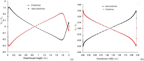
Figures 5(a) and 5(b) illustrate trends of the normalised mean velocity components $\left[v_{x}^{*}=v_{x} / v_{c}, v_{y}^{*}=v_{y} / v_{c}\right]$ along the mid-height and mid-width of the greenhouse, and $\left(v_{c}=\sqrt{g \cdot \beta \cdot \Delta T \cdot H}\right)$ being the characteristic velocity of the naturel convective flow. The bifurcations in Figure 5 are explained by the reversing of the velocity direction of the flow as observed in Figures 4(a) and 4(b), clockwise or counter clockwise, respectively and the results are virtually identical one way or the other. This phenomenon, also observed experimentally by Benkhelifa and Penot [33] and Lamrani et al. [30], is mainly due to the initial conditions, which generate perturbations within the computational process.
Figure 4. Interchangeability of the flow and thermal fields
Figure 5. Distribution of the normalised means velocity profiles. (a) Horizontal profile of the vertical normalised mean velocity component. (b) Vertical profile of the horizontal normalised mean velocity component
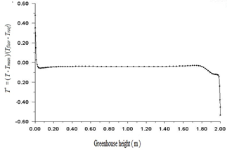
Similar to isotherms of Figure 4, the trend of the normalised temperature in the median of the greenhouse, against the vertical location, could be used to highlight the thermal behaviour, as showed in Figure 6. The normalised temperature being $T^{*}=\left(T-T_{\text {mean }}\right) /\left(T_{\text {floor }}-T_{\text {roof }}\right)$, where $T_{\text {mean }}=\left(T_{\text {floor }}+T_{\text {roof }}\right) / 2$ being the arithmetic mean temperature of the floor and roof being.
From the heated floor, the air temperature decreases on the first 2.5% of the height, remains almost uniform on the afterward 85% and decreases on the last 12.5% below the roof. This trend is in agreement with the results reported by Lamrani [26].
Figure 6. Vertical profile of the normalised temperature at the median plane
3.2 Effects of the Rayleigh number
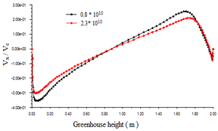
Figure 7 illustrates the trends of the normalised velocity $v_{x}^{*}=v_{x} / v_{c}$ against the vertical locations in the mid-width of the greenhouse for two Rayleigh numbers, 2.3´1010 and 0.8´1010. It shows that the maximum value of $v_{x}^{*}$ occurs in the vicinity of the floor (heated wall) and the roof (cooled wall). It is noted that the normalised velocity $\left(v_{x}^{*}\right)$ decreases with the increasing Rayleigh number, and with regard to the scale law the air flow velocity (vx) should increases.
Figure 7. Distribution of the normalised horizontal velocity component at the median plane of the greenhouse for two values of Ra
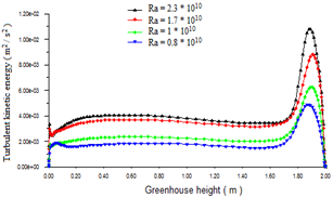
The vertical trend of the turbulent kinetic energy in the mid-width of the greenhouse is presented in Figure 8, for various values of the Rayleigh number. The turbulence field is characterized by the concentration of turbulence in the top most of the greenhouse. The rest of the flow field is almost no turbulent; the turbulences intensity increases with increasing the Rayleigh number as the velocity increases.
Figure 8. Vertical profile of the Turbulent kinetic for different heat flux densities according to Rayleigh numbers
Figure 9 is set to summarize the influence of the Rayleigh number on the normalized temperature in the mid-width. it is clear that the temperature distribution increases with the increasing of the Rayleigh number.
Figure 9. Influence of Ra number on the normalized temperature profile in mid-height cavity
3.3 Interaction of the natural convection and the surface radiation
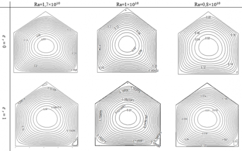
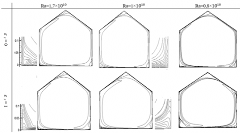
In order to understand the significance and role of the surface radiation, the wall emissivity $\left(\varepsilon_{r}\right)$ are set to 1. The effect of radiation was studied by comparing the results obtained with $\varepsilon_{r}=1$ and $\varepsilon_{r}=0$. Figures 10 and 11 show the effects of the increasing Rayleigh number on the fluid flow structures and temperature distribution inside the greenhouse with and without radiation heat transfer. The increase of the Rayleigh number which explains that the heat transfer is accentuated. The increase of convective heat would lead to buoyancy force growing which means an increase in the air velocity and consequently, the extraction of a larger heat quantity.
As a result, the isotherms and streamline structures do not change considerably when it is taken into account the radiation heat exchange, being the gas radiations are neglected and assuming it as perfectly transparent to the thermal radiation. So, only solid surfaces are concerned by thermal radiation exchange, the temperature levels of the floor heating (under a constant heat flux) / roof cooling (mixed flow condition) decrease further, which further dampens the natural convection, and this is clear, at Ra=1.7´1010, the reduction of the maximum stream function value from 0.360 $\left(\varepsilon_{r}=0\right)$ to 0.22 $\left(\varepsilon_{r}=1\right)$. In addition, the isotherms structures near the solid surfaces are affected by the thermal radiation; consequently, they are distorted near the adiabatic ones as a result of important radiations, while they are perpendicular for the pure natural convection.
Mainly, there are not qualitative changes of the streamlines taking into account or not the surface radiation, nevertheless the intensity of flow is affected.
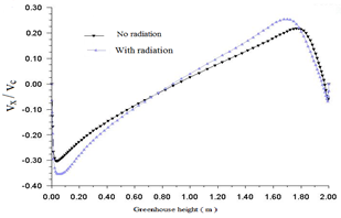
The maximum $\left|v_{x}\right|$ and $\left|v_{y}\right|$ decrease at Ra=1010 when taking into account the radiations, as showed in Figure 12 (the increase of the ratios $v_{y / v_{c}}$ and $v_{x / v_{c}}$).
The distribution of the normalised temperature of air along the mid-width of the enclosure is depicted in Figure 13, for Ra=1010. It is clear that without radiation, the overall temperature level of the walls and air is huge than with radiation (e.g., thermal radiation reduced the air temperature, the difference temperature between the horizontal walls (floor/roof) and the sidewalls (left/right).
Figure 10. Streamlines for different Rayleigh numbers with and without radiative heat transfer
Figure 11. Isotherms (a) without and (b) with radiative heat transfer
Figure 12. Normalised horizontal velocity component at mid- width of the greenhouse for Ra =1010 with and without radiation
Figure 13. Vertical profile of the reduced temperature with and without heat transfer radiation
3.4 Nusselt number
The total heat transfer involves both the convective and radiative heat transfer coefficients effects. Thus, the total Nusselt number can be expressed as:
$N u_{t o t}=N u_{\text {conv }}+N u_{r a d}$ (10)
The average Nusselt numbers of the convective and radiation heat transfer on the hot wall at y = H/2 are given as follows:
$N u_{\text {conv }}=\frac{q_{\text {conv }}(\mathrm{H} / \mathrm{2})}{K\left(T_{f}-T_{a}\right)}$ (11)
$N u_{r a d}=\frac{q_{r a d}(H / 2)}{K\left(T_{f}-T_{a}\right)}$ (12)
where, Tf being the average temperature of the floor, expressed as:
$T_{f}=\frac{1}{L} \int_{0}^{L} T(x, 0) \cdot d x$ (13)
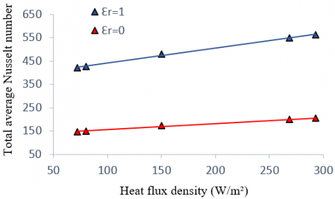
Effects of the wall thermal radiation on the average total Nusselt number of the various heat flux densities (qhf) corresponding to various Rayleigh numbers (Ra) are shown in Figures 14. In both situations, with and without thermal radiations, the average total Nusselt number increase with increasing the Rayleigh number, the heat transfer is enhanced as the Rayleigh number becomes important.
Figure 14. Total means Nusselt number with and without radiation along the floor
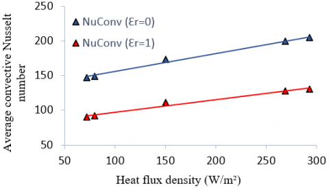
Figure 15. Means convective Nusselt number with and without coupling along the floor
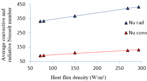
Figure 16. Means radiative and convective Nusselt number with coupling along the floor
The contribution of thermal radiation in the total heat transfer is very important, the average total Nusselt number, from Figure 14. is twice and more than in the presence of thermal radiation. Comparing the change of average convective Nusselt number during pure convection $\left(\varepsilon_{r}=0\right)$ with the mixed convection-radiation $\left(\varepsilon_{r}=1\right)$, as shown in Figure 15. It is clear that surface radiation reduces the natural convection effect on the floor. This result is due to an overall reduction in the convective flow, which is a consequence of the reduction in the difference temperature between the hot floor (under a constant heat flux)/cold roof (mixed flow condition). This reduction in the convection effect is principally compensated by the contribution of radiation as shown in Figure 16.
This result allows us to affirm that the radiative heat transfer should not be neglected in this kind of problems, otherwise significant under estimations in the total heat transfer shall be found.
This study showed the effect of the radiation heat transfer on the dynamic and thermal structure of the airflow inside the empty greenhouse enclosures with the hot bottom wall under a constant heat flux is done and consideration of mixed flow condition from the outside of the roof.
In order to evaluate the effect of the radiation exchange, both cases (pure turbulent natural convection and turbulent natural convection combined with thermal radiation) are investigated and compared. The following conclusions can be given:
The literature review showed that the majority of the studies take into account only of the convective heat transfer, while in fact, the thermal radiation has an important effect on the heat transfer inside the greenhouse, and simulations that include radiation are more realistic; it is impossible in practice to have surfaces with zero emissivity.
As perspective, in our future studies, we intend to take into account: (1) the heat exchange between the greenhouse and the surrounding environment as well as radiation from the sun and sky, (2) the impact of moisture from the air and the presence of CO2.
|
Parameters |
|
|
A Cp |
$A=L / H$, aspect ratio Specific heat [ ] |
|
$C_{\varepsilon 1},$ $C_{\varepsilon 2,} C_{\varepsilon 3}$ |
Constants in the turbulence model |
|
h |
Heat transfer coefficient, $\left[W \cdot m^{-2} \cdot K^{-1}\right]$ |
|
H |
Height of the greenhouse, $[\mathrm{m}]$ |
|
L |
Length of the greenhouse, $[\mathrm{m}]$ |
|
g |
Acceleration due to gravity, $\left[\mathrm{m} . \mathrm{s}^{-2}\right]$ |
|
K |
Turbulent kinetic energy, $\left[\mathrm{m}^{2} \cdot \mathrm{s}^{-2}\right]$ |
|
q |
Heat flux density $\left[\mathrm{W} \cdot \mathrm{m}^{-2}\right]$ |
|
qhf |
Heat flux density released by the heating film $\left[\mathrm{W} \cdot \mathrm{m}^{-2}\right]$ |
|
Nuconv |
Mean convection Nusselt number |
|
Nurad |
Mean radiation Nusselt number |
|
Nutot |
Total Nusselt number, Nuconv + Nurad |
|
Pr |
Prandtl number |
|
Ra |
Rayleigh number: $R a=g \beta q H^{4} / \lambda \alpha v$ |
|
T |
Temperature $[\mathrm{K}]$ |
|
T0 |
Reference temperature |
|
T* |
Dimensionless temperature, [-] |
|
vc |
Characteristic velocity of the air $\left[\mathrm{m} \cdot \mathrm{s}^{-1}\right]$ |
|
vx, vy |
Velocity components, $\left[\mathrm{m} \cdot \mathrm{s}^{-1}\right]$ |
|
x, y |
Dimensional coordinates, [m] |
|
Greek symbols |
|
|
$\rho$ |
Density, $\left[\mathrm{kg} \cdot \mathrm{m}^{-3}\right]$ |
|
$\alpha$ |
Thermal diffusivity, $\left[\mathrm{m}^{2} \cdot \mathrm{s}^{-1}\right]$ |
|
$\beta$ |
Thermal expansion coefficient, $\left[\mathrm{K}^{-1}\right]$ |
|
$\mu$ |
Dynamic viscosity, $\left[\mathrm{kg} \cdot \mathrm{m}^{-1} \cdot \mathrm{s}^{-1}\right]$ |
|
$\lambda$ |
Thermal conductivity, $\left[\mathrm{W} \cdot \mathrm{m}^{-1} \cdot \mathrm{K}^{-1}\right]$ |
|
$\mu_{t}$ $\sigma_{k}$ $\sigma_{\varepsilon}$ |
Turbulent viscosity, $\left[\mathrm{kg} \cdot \mathrm{m}^{-1} \cdot \mathrm{s}^{-1}\right]$ Turbulent Prandtl number for k Turbulent Prandtl number for $\mathcal{E}$ |
|
$\mathcal{E}$ |
Dissipation rate of the turbulent kinetic energy $\left[m^{2} \cdot s^{-3}\right]$ |
|
$\varepsilon_{r}$ |
Emissivity of the wall surface, [-] |
|
$\sigma$ |
Stefan–Boltzmann constant, $5.670 \times 10^{-8} \mathrm{~W} \cdot \mathrm{m}^{-2} . \mathrm{K}^{-4}$ |
|
Subscript |
|
|
a |
Air |
|
conv |
Convective |
|
ext |
external |
|
h |
Hot wall |
|
rad |
Radiative |
|
s |
Surface |
|
tot |
Total |
[1] Boulard, T. (1996). Caractérisation et modélisation du climat des serres : applications à la climatisation estivale, Doctoral dissertation. École Nationale Supérieure Agronomique, Montpellier, 1-157. (in French).
[2] Kittas, C. (1980). Contribution théorique et expérimentale à l'étude du bilan d'énergie des serres (Doctoral dissertation, Thèse Docteur-Ingénieur. Université de Perpignan, (in French).
[3] Nisen, A. (1969). L'éclairement naturel des serres. Presse Agronomique, Gembloux, (in French).
[4] Baille, M., Baille, A. (1990). A simple model for the estimation of greenhouse transmission: Influence of structures and internal equipment. In Second Workshop on Greenhouse Construction and Design, 281: 35-46. https://doi.org/10.17660/ActaHortic.1990.281.3
[5] Nijskens, J., Deltour, J., Coutisse, S., Nisen, A. (1985). Radiation transfer through covering materials, solar and thermal screens of greenhouses. Agricultural and Forest Meteorology, 35(1-4): 229-242. https://doi.org/10.1016/0168-1923(85)90086-3
[6] Kimball, B.A. (1986). A modular energy balance program including subroutines for greenhouse and other latent devices. Agricultural Research Service.
[7] Monteil, C., Issanchou, G., Amouroux, M. (1991). Modèle énergétique de la serre agricole. Journal de Physique III, 1(3): 429-454. https://doi.org/10.1051/jp3:1991130
[8] Mistriotis, A., Arcidiacono, C., Picuno, P., Bot, G.P.A., Scarascia-Mugnozza, G. (1997). Computational analysis of ventilation in greenhouses at zero-and low-wind-speeds. Agricultural and Forest Meteorology, 88(1-4): 121-135. https://doi.org/10.1016/S0168-1923(97)00045-2
[9] Boulard, T., Haxaire, R., Lamrani, M.A., Roy, J.C., Jaffrin, A. (1999). Characterization and modelling of the air fluxes induced by natural ventilation in a greenhouse. Journal of Agricultural Engineering Research, 74(2): 135-144. https://doi.org/10.1006/jaer.1999.0442
[10] Haxaire, R. (1999). Caractérisation et modélisation des écoulements d'air dans une serre. Ph.D. thesis, University of Nice Sophia Antipolis, Nice.
[11] Montero, J.I., Munoz, P., Anton, A., Iglesias, N. (2005). Computational fluid dynamic modelling of night-time energy fluxes in unheated greenhouses. Acta Horticulturae, 691: 403-410. http://dx.doi.org/10.17660/ActaHortic.2005.691.48
[12] Lee, I.B., Short, T.H. (2000). Two-dimensional numerical simulation of natural ventilation in a multi-span greenhouse. Transactions of the ASAE, 43(3): 745-753. http://dx.doi.org/10.13031/2013.2758
[13] Bournet, P.E., Ould Khaoua, S.A., Boulard, T. (2007). Numerical prediction of the effect of vents arrangement on the ventilation and energy transfer in a multispan glasshouse using a bi-band radiation model. Biosystems Engineering, 98(2): 224-234. https://doi.org/10.1016/j.biosystemseng.2007.06.007
[14] Morille, B., Migeon, C., Bournet, P.E. (2013). Is the Penmane-Monteith model adapted to predict crop transpiration under greenhouse conditions? Application to a New Guinea Impatiens crop. Scientia Horticulturae, 152: 80-91. https://doi.org/10.1016/j.scienta.2013.01.010
[15] Nebbali, R., Roy, J.C., Boulard, T. (2012). Dynamic simulation of the distributed radiative and convective climate within a cropped greenhouse. Renewable Energy. 43: 111-129. http://dx.doi.org/10.1016/j.renene.2011.12.003
[16] Ould Khaoua, S.A., Bournet, P.E., Chassériaux, G. (2006). Mathematical modelling of the climate inside a glasshouse during daytime including radiative and convective heat transfers. In III International Symposium on Models for Plant Growth, Environmental Control and Farm Management in Protected Cultivation, 718: 255-262. http://dx.doi.org/10.17660/ActaHortic.2006.718.28
[17] Tong, G., Christopher, D.M., Li, B. (2009). Numerical modelling of temperature variations in a Chinese solar greenhouse. Computers and Electronics in Agriculture, 68(1): 129-139. http://dx.doi.org/10.1016/j.compag.2009.05.004
[18] Fatnassi, H., Boulard, T., Ravel, O., Roy, J. (2012). CFD simulation of climate conditions in an ecotron dedicated to ecosystem studies in the context of environmental changes: preliminary results. Acta Horticulturae (ISHS), 952: 177-183. http://dx.doi.org/10.17660/ActaHortic.2012.952.21
[19] Roy, J.C., Vidal, C., Fargues, J., Boulard, T. (2008). CFD based determination of temperature and humidity at leaf surface. Computers and Electronics in Agriculture, 61(2): 201-212. http://dx.doi.org/10.1016/j.compag.2007.11.007
[20] Majdoubi, H., Boulard, T., Fatnassi, H., Bouirden, L. (2009). Airflow and microclimate patterns in a one-hectare Canary type greenhouse: An experimental and CFD assisted study. Agricultural and Forest Meteorology, 149(6-7): 1050-1062. http://dx.doi.org/10.1016/j.agrformet.2009.01.002
[21] Qian, T., Dielman, J.A., Ehling, A., Marcelis, L.F.M. (2015). Response of tomato crop growth and development to a vertical temperature gradient in a semi-closed greenhouse. Journal of Horticultural Science and Biotechnology, 90(5): 578-584. https://doi.org/10.1080/14620316.2015.11668717
[22] Boulard, T., Roy, J.C., Pouillard, J.B., Fatnassi, H., Grisey, A. (2017). Modelling of micrometeorology, canopy transpiration and photosynthesis in a closed greenhouse using computational fluid dynamics. Biosystems Engineering, 158: 110-133. http://dx.doi.org/10.1016/j.biosystemseng.2017.04.001
[23] Henkes, R.A.W.M., Hoogendoorn, C.J. (1995). Comparison exercise for computations of turbulent natural convection in enclosures. Numerical Heat Transfer, Part B, 28(1): 59-78. http://dx.doi.org/10.1080/10407799508928821
[24] Xu, W., Chen, Q., Nieuwstadt, F.T.M. (1998). A new turbulence model for near-wall natural convection. International Journal of Heat and Mass Transfer, 41(21): 3161-3176. http://dx.doi.org/10.1016/S0017-9310(98)00081-7
[25] Markatos, N.C., Pericleous, K.A. (1984). Laminar and turbulent natural convection in an enclosed cavity. International Journal of Heat and Mass Transfer, 27(5): 755-772. http://dx.doi.org/10.1016/0017-9310(84)90145-5
[26] Barakos, G., Mitsoulis, E., Assimacopoulos, D. (1994). Natural convection flow in a square cavity revisited: laminar and turbulent models with wall functions. International Journal for Numerical Methods in Fluids, 18(7): 695-719. http://dx.doi.org/10.1002/fld.1650180705
[27] Henkes, R.A.W.M. (1990). Natural Convection Boundary Layers. Ph.D. thesis, Delft University of Technology, Netherlands.
[28] Siegel, R., Howell, J.R. (2002). Thermal Radiation Heat Transfer.
[29] Modest, M.F. (2013). Radiative Heat Transfer. Third ed. Academic Press, New York.
[30] Lamrani, M.A., Boulard, T., Roy, J.C., Jaffrin, A. (2001). Structures and environment: Airflows and temperature patterns induced in a confined greenhouse. Journal of Agricultural Engineering Research, 78(1): 75-88. http://dx.doi.org/10.1006/jaer.2000.0568
[31] Jolliet, O., Danloy, L., Gay, J.B., Munday, G.L., Reist, A. (1991). Horticern: an improved static model for predicting the energy consumption of a greenhouse. Agric Forest Meteorol, 55(3-4): 265-294. http://dx.doi.org/10.1016/0168-1923(91)90066-Y
[32] Papadakis, G., Frangoudakis, A., Kyritsis, S. (1992). Mixed, forced and free convection heat transfer at the greenhouse cover. J Agric Engng Res, 51: 191-205. http://dx.doi.org/10.1016/0021-8634(92)80037-S
[33] Benkhelifa, A., Penot, F. (2006). Sur la convection de Rayleigh-Bénard turbulente: Caractérisation dynamique par PIV. Revue des Energies Renouvelables, 9(4): 341-354.