Ahmed Abed Al-Kadhem Majhool* | Noor Mohsin Jasim
© 2020 IIETA. This article is published by IIETA and is licensed under the CC BY 4.0 license (http://creativecommons.org/licenses/by/4.0/).
OPEN ACCESS
The polydispersed nature of the spray is captured through the use of probability density functions based on the maximum entropy method to stand for the complete atomization characteristics of spray dynamics. The droplet and velocity size distributions are practical tools for the analysis of sprays cooling. The special benefit of the model is a Eulerian based which is less computationally intensive when compared to models that are based on the Lagrangian approach that tracks droplet parcel. The accuracy of using Lagrangian approach in polydispersed phase is always accurately less than Eulerian approach because it depends on the number of parcels while in Eulerian approach it depends on the proposed continuous distribution function. The main intent of the current work is to evaluate the capability of using the model for the initial predictions of the droplet size and velocity distribution for liquid nitrogen spray of solid-cone pressure swirl nozzle. The use of liquid injection pressure cases of up to 0.6MPa and spray cone angles of just 30◦ from three different sets of experimental data. The results being characterized are spray drop size distribution, liquid volume fraction and spray cone angle values. The unsteady analyses of the effect of injection pressure are studied on the cryogenic liquid nitrogen. The numerical results show that the maximum entropy method applies to liquid cryogenic spray and indicates that the model reacts correctly to changes in different injection pressures. Comparisons are also made with measured drop size distribution data that are reasonably captured and the spray cone angle is found to be in good agreement during initial and far-field spray angles.
spray modeling, liquid cryogenic spray, probability density function, maximum entropy method, droplet velocity
There are similarities between regimes and physical phenomena highlighted in the cases of bath cooling and spray cooling [1]. However, these two types are fundamental differences in cooling. On the one hand, a spray is discontinuous and consists of two phases and secondly, spray cooling depends on both the distribution of the liquid flow in space and the specific characteristics of droplets (probability density function of droplet diameters and velocity among other characteristics). These specificities are responsible for mechanisms specific to the interaction between a spray and a hot plate. Under certain cooling conditions, the liquid film takes the shape of the surface. The conditions of appearance of this film generally require a large surface flow and the impact surface large enough for the film to develop and conditions particular thermal. This liquid film is not necessarily continuous, the surface of the plate is presented as a succession of liquid or dried zones. The definition of the two spray cooling configurations. First, the direct impact where the plate is dry or just wet. The drops impact directly the surface and heat transfer takes place either directly between the surface and the drop deformed by the impact on the wall, either through the film of vapor forming between the deformed drop and the wall of the case of Leidenfrost. Second, the impact on a liquid film when the plate is then embedded by the spray. Drops impact the liquid film, but the heat transfer is caused by several phenomena: convection by the liquid film, direct evaporation, boiling and impact of drops. A numerical study was implemented by Zhang et al. [2] to simulate the cavitation phenomena in liquid nitrogen. The case of the study had used a flow through ogives and hydrofoils. They assumed that there is a thermal equilibrium between the liquid phase and the vapor phase through the thermodynamic analysis. They also were investigated the choking phenomenon with high Mach number. Both experimental and numerical work of the micro-slush jet of a two-fluid nozzle were analyzed and examined by Ishimoto [3]. The atomization and flow characteristics were studied using micro-slush nitrogen particles in a two-fluid nozzle. The numerical analyses were considered a superadiabatic two-fluid ejector nozzle approach, where the nozzle is capable of handling with generating and atomizing micro-slush nitrogen spray under pressurized subcooled conditions. The effects of many important factors, such as the surface geometry, jet velocity, the nozzle geometry exit and condition of heat transfer surface investigated experimentally by Zhang et al. [4]. Their investigation was carried out onto different heat transfer surface geometries and conditions on the confined jet impingement using liquid nitrogen issuing from a tube of onto the heat transfer surfaces. Experimental and numerical simulation were carried out by Ishimoto et al. [5]. The Eulerian-Lagrangian model was used to simulate the atomization of cryogenic spray micro-solid nitrogen particles. The model was applied for the spray impingement on a heated substrate to study a sort of ultra-high heat flux cooling system. They found that when micro-solid nitrogen particles are used give better cooling performance than liquid nitrogen. For some applications, liquid nitrogen spray is used as a coolant. It can be considered a good option of an open cooling system. However, Somasundaram and Tay [6] were used liquid nitrogen sprays in their experimental steady-state measurements for intermittent spray cooling under different temperature ranges to coverall zones. Their work was carried out under different ranges of surface temperatures (-180C to 20C). Liu et al. [7] experimentally studied the effect of various injection pressure on the spray cone angle and the drop size distribution. Their work used a liquid nitrogen spray as a working fluid in the cooling system. The measurements showed that the spray cone angle is unresponsive to the varying injection pressure differences. Nevertheless, when the flow is developed far away from the injector, the spray cone angle decreases rapidly with increasing the injection pressure difference. Liu et al. [8] experimentally studied the injected liquid nitrogen spray through solid-cone pressure swirl nozzles. The experimental apparatus of the liquid nitrogen spray cooling system was built. The outcome of different injection pressure on the flow patterns of liquid nitrogen spray was analyzed and compared with that of water. The measurements also displayed that the mass flow rate of liquid nitrogen spray is less than for water in all range of injection pressure difference. The discharge coefficient of water decreases and increases for liquid nitrogen while the injection pressure difference increases. Computational fluid dynamics simulations were done by Xue et al. [9]. To study the cavitation phenomena of spray liquid nitrogen over hydrofoil. A mixture model is used to simulate liquid nitrogen spray under different inlet temperature and pressure. Their results showed that the nozzle outlet diameter, the inlet temperature, and pressure difference have significantly influenced the mass flow rate of spray droplets. The change of the inlet temperature leads to a change in saturation pressure which leads to an increase in cavitation intensity and generates more vapor at nozzle orifice, which reduces mass flow rate. The effect of the thermophysical properties of cryogenic liquid in the cavitating flow was studied numerically by Xue et al. [10]. The geometrical parameters through a spray nozzle had been also used in the study which has a strong effect on the cavitating flow. Xue et al. [11] proposed a numerical model to study the cavitating flow of liquid nitrogen using spray nozzles at different temperatures. Their study was based on the effect of fluctuations of inlet pressure, amplitude, and frequency on the spray cavitation. The results showed that the cavitation flow can be reduced slightly when the frequency is increased and enhanced with pressure fluctuating. The thermal effect of the cavitating flow of liquid nitrogen around two-dimensional hydrofoil was reported numerically by Zhang et al. [12]. The RNG k-ε turbulence model with a modified turbulent eddy viscosity was used with the coupled energy equation to express the thermal effects. In addition, the homogenous cavitation model was conjugated with the energy equation. An extension for the Zwart-Gerber-Belamri model was considered to describe the convection heat transfer. The temperature and pressure were calculated under cryogenic conditions. According to Li et al. [13] had numerically simulated a liquid nitrogen jet. The cryogenic fluid is injected and mixed under transcritical and supercritical conditions. The open-source software OpenFOAM was used to explain the differences between the cases, especially on the mechanism and characteristics. The numerical results were showed that there are differences between transcritical and supercritical conditions when injectors were induced by the pseudo-boiling phenomenon. Also, the results were demonstrated that a longer penetration of cold liquid core is found with transcritical jet. In contrast, an isothermal expansion occurs at the surface rather than the volume of the cold-core. Extensive research was conducted on the characteristics at the macroscopic and microscopic properties of liquid nitrogen spray that was performed by Xue et al. [14]. The liquid nitrogen spray was injected through a nozzle at ambient temperature with different outside diameters. The application was used as an open cycle in a cooling system. Moreover, Xue et al. [15] showed in their study, the influence of different injection pressures on the nozzle inside diameter, the mass flow rate, drop size distribution, discharge coefficient, spray flow pattern, and spray cone angle were studied. Most recently, Wang et al. [16] were conducted theoretical analysis and numerical study liquid nitrogen spray as a cryogenic cooling fluid in electronic equipment under low pressure. The energy analyses use the First Law of Thermodynamics in the heat balance equation. The spray cooling model is implemented with a thermal control strategy for a semi-cavity electronic device. This strategy benefits from switching and the action performance between pressure and temperature. In designing the spray cooling system which is used in the cryogenic wind tunnels an experimental and numerical studies were performed by Ruan et al. [17]. The effect of droplet mass flow rate, droplet velocity, droplet diameter, and injection pressure were investigated as design parameters of the droplet evaporation and droplet size distribution of liquid nitrogen. The main difficulty that has been encountered between the two approaches that an ordinary differential equation (Lagrangian framework) or transport equations (Eulerian framework) are not needed to be solved for the conservation of quantity, momentum and energy. The application of the maximum entropy formalism to sprays consists of calculating drop size distributions that satisfy constraints that the physics of atomization processes impose and for which entropy is maximized Sellens and Brzustowski [18] and Cao [19]. The mathematical model of the drop size distribution of the spray was determined at starting from the mathematical function developed within the laboratory by Dumouchel [20]. This function is the solution to the application of the maximum entropy formalism applied to sprays. This mathematical solution is suitable to represent a large number of experimental distributions. Indeed, this solution covers the distribution of Rosin-Rammler and is identical to the distribution of Nikiyama-Tanasawa [21]. This mathematical solution has also been successfully used to reproduce distributions of drop size of sprays produced by different types of injectors Lecompte and Dumouchel [22]. The moments method of polydisperse phase describes multiphase flows based on the transport equation of moments of the droplet size distribution function [23, 24]. The droplet size of the droplet velocities is evaluated by transporting the moments with individual moment transport velocities [25]. Laurent et al. [26] applied the quadrature method of moments method in the characterization of continuous mixtures in the vaporization processes of a drop of kerosene and compared the results with a characterization of the mixture through the Gamma function and with a complete multi-component case. They derived the moment conservation equations for the case studied and demonstrate that it is possible to obtain results similar to the complete multicomponent model with the quadrature method of moments (QMOM), but with a reduction in computational cost. This work addresses the improvement of a statistical means for predicting the initial distribution of the droplet size and velocity of liquid nitrogen spray injected into the atmosphere. The Maximum Entropy Method is a statistical way that permits the prediction of a probability distribution that is consistent with information from the input data system.
Spray atomization issued from the single injector is the result of a bulk of liquid, which develops instabilities, breaks up and collides into ligaments and finally forms droplets. The droplet formation process in each control volume can be considered as an equilibrium state that is transferred from one state to another control the droplet size distribution and droplet velocity distribution. Reported by the thermodynamics conservation laws, mass, momentum, and energy are conserved as well as entropy maximization during the change in the process occurs. The set of constraints that are developed to include breakup, collision and spray evaporation are practically conservative processes. The set of conservation equations downstream of spray atomization can be presented as the probability density function p, which is the probability of determination droplets based on both droplet diameter D, droplet velocity vd and droplet volume Vd [27]. This approach is assumed that the spray droplets formed after injecting from the nozzle just downstream. The spray atomization processes such as breakup and collision area have the same total mass, momentum, surface energy, and entropy. Maximum Entropy Principle (MEP) is used the consideration of an equally spaced and normalized size and velocity space. All constraints are solved to comprise both of these variables so that dp=dvdD. To solve the computational domain dϕ must have both v, droplet velocity, and D, droplet diameter. According to Cao [19] the probability density function principle, the total summation of for any distribution function is equal to unity. Probability density functions are used for droplet size and velocity distributions. Governing equations of liquid mass, momentum, and energy have to satisfy through the atomization process. They are modeled for a control volume. The computational domain extends from the nozzle exit plane towards the regime of spray droplets formation. The conservation equations are concerned with the entropy maximization principle and can be written based on the probability density function. Therefore, the governing equations can be written as:
$\sum_{i} \sum_{j} p_{i j} V_{i} \rho \dot{n}=\dot{m}_{o}+S_{m}$ (1)
$\sum_{i} \sum_{j} p_{i j} V_{i} \rho u_{j} \dot{n}=j_{o}+S_{m u}$ (2)
$\sum_{i} \sum_{j} p_{i j} \dot{n}\left(V_{i} \rho u_{j}^{2}+2 \sigma A_{i}\right)=\dot{E}_{o}+S_{e}$ (3)
where, $\dot{n}$ is the total number of droplets are formed per unit time and also $\dot{m}_{o}, j_{o} \text { and } \dot{E}_{o}$ are the mass flow rate, momentum, and energy that enter the computational domain from the injector orifice respectively. uj, σ and Ai are the droplet velocity, surface tension and liquid contact area, respectively. Sm, Smu and Se are the source terms of mass, momentum, and energy equations, respectively. In addition, the sum of probabilities has to be equal to unity, constraint develops from the definition of a probability is:
$\sum_{i} \sum_{j} p_{i j}=1$ (4)
There are many numbers of probability distribution functions (pij) which could satisfy Eqns. (1) to (3), but the most applicant and proper function is that can fit the maximum entropy principle states for all these possibilities. The most objective distribution is Shannon entropy [28]:
$S=-K \sum_{i} \sum_{j} p_{i j} \ln \left(p_{i j}\right)$ (5)
where, K is the Boltzmann constant. The solution domain is converted to diameter and velocity instead of volume and velocity of droplets. Then, the equations can be transformed according to the probability function of being proposed as the droplets whose diameters change from $\bar{D}_{n-1} \text { and } \bar{D}_{n}$ and that velocities change from $\bar{u}_{m-1} \text { and } \bar{u}_{m}$. Then, Eqns. (1) to (3) can be transformed as a non-dimensional and integral forms within the computational domains of diameter and velocity of the droplet and written in the form of equations:
$\int_{\bar{D}_{\min }}^{\bar{D}_{\max }} \int_{\bar{u}_{\min }}^{\bar{u}_{\max }} f \bar{D}^{3} d \bar{u} d \bar{D}=1+\bar{S}_{m}$ (6)
$\int_{\bar{D}_{\min }}^{\bar{D}_{\max }} \int_{\bar{u}_{\min }}^{\bar{u}_{\max }} f \bar{D}^{3} \bar{u} d \bar{u} d \bar{D}=1+\bar{S}_{m u}$ (7)
$\int_{\bar{D}_{\min }}^{\bar{D} \max } \int_{\bar{u}_{\min }}^{\bar{u}_{\max }} f\left(\bar{D}^{3} \bar{u}^{2}+B \bar{D}^{2}\right) d \bar{u} d \bar{D}=1+\bar{S}_{e}$ (8)
$\int_{\bar{D}_{\min }}^{\bar{D}_{\max }} \int_{\bar{u}_{\min }}^{\bar{u}_{\max }} f d \bar{u} d \bar{D}=1$ (9)
To solve Eqns. (6) to (9), a non-dimensional form of probability function that uses Lagrange multipliers to maximize Shannon entropy (Eq. (5)) and satisfy the constraints given in conservation equations is represented as:
$\begin{array}{r}
f=3 \bar{D}^{2} \exp \left[-\lambda_{o}-\lambda_{1} \bar{D}^{3}-\lambda_{2} \bar{D}^{3} \bar{u}-\lambda_{3}\left(\bar{D}^{3} \bar{u}^{2}\right.\right. \\
\left.\left.+B \bar{D}^{2}\right)\right]
\end{array}$ (10)
where, the set of λi (i=0, 1, 2, 3) are the Lagrange multipliers that have to be determined from solving the Eqns. (6) to (8) simultaneously. The Newton–Raphson method is used to solve equations set and then the probability function is computed by Eq. (10). The computational domains for nondimensional diameter and velocity are assumed to be varied from 0 to 1. In the present modeling, the continuity source term is not set to zero implying that the cooling during the atomization is considered. However, it should be mentioned that the energy source term is due to the energy transformation inside the control volume and is regarded as a source term. Additionally, the effect of exchange between the gas and spray droplets flow in the control volume due to drag force and the breakup of droplets is considered in the momentum equations as a momentum source term. The dimensionless diameter, velocity, source terms and other parameters in these equations are written as:
$W e=\frac{\rho \bar{u}^{2} D_{30}}{\sigma}, B=\frac{12}{W e}$ (11)
$\bar{D}_{i}=D_{i} / D_{m,} \bar{u}_{j}=u_{j} / \bar{u}_{o}$ (12)
$\bar{S}_{m}=S_{m} / \dot{m}_{o}, \bar{S}_{m u}=S_{m u} / \dot{\jmath}_{o}, \bar{S}_{e}=S_{e} / \dot{E}_{o}$ (13)
where, B is a constant and is related to the surface tension. We and D30 are the Weber number and the volume mean diameter of droplets and is calculated using the following equation:
$D_{30}=\frac{\sum n_{i} d_{i}^{3}}{\sum n_{i}}$ (14)
3.1 Droplet breakup model
For the discrete phase, the Wave model is selected as the breakup model because it is suitable for high injection velocity when the Weber number is larger than 100. The model assumes the breakup of the droplets to be induced by the relative velocity between the liquid and gas phases. The wave breakup model is based on the study of the linear instability of a column of liquid injected into an incompressible gaseous environment. It assumes that the atomization is due to the development of surface instabilities of type Kelvin-Helmholtz at the exit of the injector. This model consists of representing the column of liquid by more or less spherical liquid particles (“blobs”), initially of diameter equal to the orifice injection. The number of particles created by no calculation time is determined according to the liquid fuel flow [29]. The linear analysis allows to determine the wavelength ΛKH, as well as its rate of increase ΩKH. The wavelength and growth rate of this instability are used to predict the newly-breakup formed droplets. The following expressions are obtained after theoretical studies on the behavior of dimensionless numbers of Ohnesorge and Weber:
$\frac{\Lambda_{K H}}{r_{i}}=9.02 \frac{(1+0.45 \sqrt{O H})\left(1+0.4 T a^{0.7}\right)}{\left(1+0.865 W e^{1.67}\right)^{0.6}}$ (15)
$\Omega_{K H} \sqrt{\frac{\rho_{l} r_{1}^{3}}{\sigma_{l}}}=\frac{0.34+0.385 \mathrm{W} e^{1.5}}{(1+0 h)\left(1+0.4 T a^{0.6}\right)}$ (16)
where, Ta=Oh We and r1 is the radius of the mother droplet. The mother’s droplet is called the droplet before the breakup process and droplet daughters are the droplets resulting from the mother drop after the breakup. These droplets daughters have a radius r2 determined as follows:
$r_{2}=\left\{\begin{array}{c}
B_{o} \Lambda_{K H} \quad \text { if } B_{O} \Lambda_{K H} \leq r_{1} \\
\min \left[\left(\frac{3 \pi a^{2} u_{l}}{2 \Omega_{K H}}\right)^{1 / 3},\left(\frac{3 \pi a^{2} \Lambda_{K H}}{4}\right)^{1 / 3}\right] \text { if } B_{o} \Lambda_{K H}>r_{1}
\end{array}\right.$ (17)
where, B0 is a modeling constant taken generally equal to 0.61. The particular case B0ΛKH ≤ r1 corresponds to the Rayleigh fractionation regime. Indeed, it is only in the presence of this breakup regime that drops detached from the liquid column have a larger diameter than that of the column itself. Concerning the high injection pressure, it is in the atomization regime that the liquid jet splits. So, the radius of the daughter droplets predicted by the model “Wave” will be rather of the order of magnitude of ΛKH at a modeling constant. The size of the droplet girl is thus determined by the volume of liquid contained in a wave of the surface. The size of the drops decreases during the breakup time as:
$\frac{d_{r 1}}{d t}=\frac{r_{2}-r_{1}}{\tau_{b u, K H}}$ (18)
The decrease in the size of mother droplets is linear in time. It is possible to express the breakup time τbu,KH based the wavelength ΛKH, its growth rate ΩKH and the radius of the mother droplets r1:
$\tau_{b u, K H}=3.726 B_{1} \frac{r_{1}}{\Lambda_{K H} \Omega_{K H}}$ (19)
In this work, the constant B1 fixes around 10, admitting that this value can be modified under the influence of the geometry of the injector on the spray formed in the chamber. Also, this model provides a radial velocity component for daughter droplets:
$V_{0}=U_{0} \tan \left(\frac{\theta}{2}\right)$ (20)
It is uniformly distributed between 0 and θ, angle of the spray, defined by the following relation:
$\tan \left(\frac{\theta}{2}\right)=A_{1} \Lambda_{K H} \frac{\Omega_{K H}}{U_{0}}$ (21)
where, A1 being a modeling constant that is a function of the design of the nozzle. Here, it proposes to take it equal to 0.188.
3.2 Droplet drag model
The component drag force can be considered as the force resistance exerted by the gas on the droplet to slow it down. According to the commonly used law of Schiller-Naumann, it involves the concept of the cross-section of droplet Aeff and a drag coefficient CD [30].
$F_{D}=\frac{1}{2} \rho_{l} C_{D} A_{e f f}\left(U_{l}-u_{g}\right)^{2}$ (22)
where, Ul and ug are the instantaneous velocity components of the liquid and the gas respectively. The coefficient CD is expressed from the following correlation obtained experimentally from the Stokes law:
$C_{D}$$=\left\{\begin{array}{cc}
4.093 & \text { if } \mathrm{Re}_{d} \leq 10 \\
24 \mathrm{Re}_{d}^{-1}+3.48 \mathrm{Re}_{d}^{-0.313} & \text {if } 10<\mathrm{Re}_{d} \leq 1000 \\
0.424 & \text { if } \mathrm{Re}_{d}>1000
\end{array}\right.$ (23)
and the Reynolds number is given by:
$R e_{d}=\frac{2 \rho_{g}\left(U_{l}-u_{g}\right) \mid r}{\mu_{g}}$ (24)
where, r is the droplet radius. The drag source term in the momentum equation is given by:
$\bar{S}_{m u}=\frac{F_{D}}{\rho_{l} U_{l}^{2} A_{e f f}}$ (25)
3.3 Droplet collision model
The drop collision affects the drop diameter and the drop size distribution. Interaction processes such as masses, momentum, and energy exchange between drops and gas phase can be strongly influenced by them. Therefore, the drop collision and coalescence in spray simulation are of great importance. To do this, the probability of a drop collision must first be calculated. This depends on the speed, the direction of movement and of course the drop distribution in the spray. From these conditions, it can be deduced that the probability of a drop collision must decrease from the nozzle area to the spray edge or to the spray tip penetration. The drop collision and coalescence model according to O′Rourke [31] is implemented in KIVA3V. This describes the number of drop collisions in a grid cell and, if a collision occurs, the type of drop interaction. The presented model implemented in the KIVA computer program used the Poisson distribution method to describe the probability of the number of collisions that take place between each parcel in the same control volume in one time step:
$P_{N}=\frac{\bar{n}_{N}}{N !} e^{\bar{n}}$ (26)
where, $\bar{n}$ is the average number of the collision given by:
$\bar{n}=\frac{c \pi}{V_{c e l l}}\left(r_{1}+r_{2}\right)^{2} U_{r e l} \delta t$ (27)
The collision probability can be calculated via the collision frequency, which indicates the probability of n collisions between a drop in Parcel 1 and a drop in Parcel 2. A collision occurs when the probability of no collision is less than a random number between 0 and 1. The collision frequency for the cell under consideration calculated. The indices 1 and 2 refer to the colliding parcel in the cell volume Vcell, whereby the index 2 relates to the parcel with the smaller drops. N2 indicates the number of drops in parcel 2 and r1 and r2 are the radii of the drops that move with the relative speed Urel. The interaction of the colliding drops is in turn controlled by a random number between 0 and 1. For this purpose, the critical impact parameter bkr is calculated for the drops concerned, which is calculated from the drop radius, the relative speed between the drops and the surface tension. If the random number is smaller than the critical impact parameter, the collision results in coalescence. If the value is higher, no coalescence occurs. To know whether a collision takes place a random number is taken from a uniform distribution and compared with PN. If the random variable > PN then collision is valid.
3.4 Droplet evaporation model
The evaporation of droplets of liquid is significantly influenced by the heat and mass exchange between the phases. The Spalding evaporation model is integrated into this work, which takes into account convection and the heat introduced between the drops and the gas surrounding them [32]. The rate of change of droplet radius according to Frossling correlation due to evaporation is given by:
$\frac{d r}{d t}=-\frac{\rho_{g} D_{g} B_{M} S h}{2 \rho_{l} r}$ (28)
Spalding [33] suggested that the mass transfer number is calculated from:
$B_{M} \equiv \frac{f_{s}-f}{1-f_{s}}$ (29)
and heat transfer number from:
$B_{T} \equiv \frac{c_{p f}\left(T_{\infty}-T_{s}\right)}{L\left(T_{s}\right)-Q_{L} / \dot{m}}$ (30)
where, Sh and fs denote Sherwood number and the fuel vapor mass fraction at the droplet surface respectively. QL and $\dot{\mathrm{m}}$ refer to overall heat penetrating to the droplet and mass transfer rate respectively. The Sherwood number as:
$\mathrm{Sh}=2+0.6 \mathrm{Re}^{1 / 2} \mathrm{Sc}^{1 / 3} \frac{\ln \left(1+\mathrm{B}_{\mathrm{M}}\right)}{\mathrm{B}_{\mathrm{M}}}$ (31)
where, Sc is the Schmidt number calculated from:
$S c=\frac{v}{D}$ (32)
where, ν and D are dynamic viscosity and mass diffusivity respectively. The heat transfer between droplets and gas-phase is governed by the energy balance equation. The conduction heat transfer entering to the droplets is given by:
$Q_{\text {cond}}=Q_{\text {conv}}+\dot{m} L\left(T_{d}\right)$ (33)
where,
$Q_{\text {cond}}=\frac{K\left(T_{g-} T_{d}\right)}{d} N u$ (34)
where, the Nusselt number Nu is determined from:
$\mathrm{Nu}=2+0.6 \mathrm{Re}^{1 / 2} \operatorname{Pr}^{1 / 3} \frac{\ln \left(1+\mathrm{B}_{\mathrm{M}}\right)}{\mathrm{B}_{\mathrm{M}}}$ (35)
where, Pr is the Prandtl number. The stagnant film theory was employed by Majhool [32] to calculate the droplet evaporation rate in order to solve the energy equation and fuel vapor species mass fraction, the vaporization rate is given as:
$\dot{m}=-\pi d N u D_{s} \rho_{s} \ln \left[1+\frac{f_{s}-f}{1-f_{s}}\right]$ (36)
The numerical simulation of an atomization process requires an exact capture of the complex deformations between the liquid interface and gas. The solution of these types of flows that involve atomization is complex, from defining the border between the two phases, which is unknown a prior and it has been the fundamental part of the solution. To involve the management of large density, viscosity and velocity relationships between the flows of each fluid. Many numerical techniques are developed to attack this type of problems, these can be divided based on the type of flow modeling (Eulerian, Lagrangians or mixed), to the modeling type of the interface (from capture or tracking) and the type of discretization (without mesh, finite differences, finite volume, finite element or others). The volume-of-fluid (VOF) is used in this work because of one of the typical applications of the VOF model is the stationary or transient monitoring of any liquid-gas interface [34]. In this case, liquid nitrogen and air are injected into the atmosphere. The formulation of the model is based on the introduction of a variable, α, known as “the volume fraction of the phase-in each computational cell”, this variable defines the fraction of each phase (liquid nitrogen or air) that corresponds to a certain cell. In each volume of control, the volumetric fractions of all phases add up the unit. The variables and the properties in any cell are multiplied by the volumetric fraction of each phase (water or air), in this way the following combinations are possible:
αq=0: the cell is empty of the fluid q(air) - Secondary phase.
αq=1: the cell is filled with fluid q (Liquid nitrogen)- Primary phase.
0< αq <1: the cell contains the interface between the fluid q and another fluid (Mixture of Liquid nitrogen and air on the free surface). The monitoring of the interface seeks to know the volumetric fraction of one or the other phase and it is achieved by solving an equation of continuity modified by the factor volumetric. This equation has the following form of the phase q.
$\frac{1}{\rho_{q}}\left[\frac{\partial\left(\alpha \rho_{q}\right)}{\partial t}+\frac{\partial\left(U\left(\alpha \rho_{q}\right)\right)}{\partial x_{i}}=S_{\alpha q}+\sum_{p=1}^{n}\left(\dot{m}_{p q}-\dot{m}_{q p}\right)\right]$ (37)
where, $\dot{m}_{p q}$ is the mass transfer from phase q to phase p and vice versa for $\dot{m}_{p q}$ , and Sαq is a source term. The above equation is not resolved for the primary phase. The primary phase (Liquid nitrogen) is given by as defined below:
$\sum_{q=1}^{n} \alpha_{q}=1$ (38)
One single momentum equation has been solved throughout the domain with the velocity fields shared by the two phases and is described by the equation:
$\frac{\partial(\rho \vec{v})}{\partial \mathrm{t}}+\nabla \cdot\left((\rho \vec{v} \vec{v})=-\nabla \mathrm{p}+\nabla \cdot\left[\mu\left(\nabla \vec{v}+\nabla \vec{v}^{T}\right]+\bar{S}_{m u}\right.\right.$ (39)
As far as the current knowledge is concerned, numerical models based on the two equation k-ε turbulence model. It might be the most powerful model to deal with the time-dependent flows including the atomization processes [23] and [25]. This model, in which the turbulent length scale of turbulence is determined from a transport equation. The model (k−ε) standard is the most used in the RANS simulations. This model uses two additional transport equations, one for kinetic energy turbulent, (k), and another for the viscous dissipation rate, (ε). The standard k-ε model of Launder and Spalding [35] is a Two Equation model, as already mentioned above, and thus requires two transport equations, one for k (the turbulent kinetic energy) and the other for (its turbulent dissipation rate) ε, to describe the turbulence. The low-Reynolds-number k-ε model of Launder and Sharma [36] contains certain modifications which have to be made if one wants to apply this model to near wall regions, where the Reynolds number is low. Therefore the k and ε equations are thus:
$\frac{D(\rho k)}{D t}=\frac{\partial}{\partial x_{i}}\left[\left(\mu+\frac{\mu_{t}}{\sigma_{t}}\right) \frac{\partial k}{\partial x_{i}}\right]+\rho P_{k}-\rho \epsilon$ (40)
where, Pk is the production term created by mean shear, defined as:
$P_{k}=v_{t}\left(\frac{\partial U_{i}}{\partial x_{i}}\right)$ (41)
$\frac{D(\rho \tilde{\epsilon})}{D t}=\frac{\partial}{\partial x_{i}}\left[\left(\mu+\frac{\mu_{t}}{\sigma_{\tilde{\epsilon}}}\right) \frac{\partial \tilde{\epsilon}}{\partial x_{i}}\right]+C_{\tilde{\varepsilon} 1} \rho \frac{\tilde{\epsilon}}{k} P_{k}-C_{\tilde{\varepsilon} 2} f_{\tilde{\varepsilon}} \rho \frac{\tilde{\epsilon}}{k}$ (42)
where, the turbulent viscosity equation is given by:
$\mu_{t}=\rho C_{\mu} f_{\mu} \frac{k^{2}}{\epsilon}$ (43)
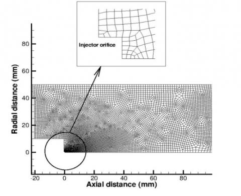
It should be noticed that all parameters and constants have the same nomination taken from the above two references with no changes. The computational domain for the liquid nitrogen spray is modeled by using an unstructured grid as shown in Figure 1. Where the constant volume (length=100mm, width=50mm). The influence of grid size on the simulation results is expressed first to select the optimum size of the grid. Therefore, the grid analysis study was carried out on different cell sizes of the grid. The inhouse-code is used GAMBIT software to generate a grid and to provide criteria for the grid refinement. The procedure is based on the increased grid resolution for the computational domain only at certain places to reduce the running time by increasing the number of cells or the compression ratio. Table 1 shows the grid specifications.
Figure 1. The computational domain
Table 1. Grid specification
|
Case |
No. vol. |
No. fac. |
No. vert. |
No. inj. cells |
|
Case A |
1906 |
3901 |
1996 |
5 |
|
Case B |
1925 |
3939 |
2015 |
5 |
|
Case C |
2011 |
4111 |
2101 |
5 |
|
Case D |
2301 |
4317 |
2318 |
5 |
|
Case E |
7799 |
15787 |
7989 |
5 |
The probability density functions (pdf) of the droplet sizes of the spray can be obtained by defining classes and counting the number (n) of droplets contained in each of these classes, then a histogram is obtained. In Figure 2 a comparison has been made between the experimental work of Liu et al. [7] and the present simulation. The two methods of discretization for drop size distribution with a size range of droplets given by a range from D-ΔD/2 to D +ΔD/2. It calculates the discretization of a probability density function of the expositional function type (Eq. 10). It should be noted that qualitatively that the two discretizations reproduce the probability density function, however, the resolution of droplets understood before the maximum of the function is better for logarithmic discretization. It must be remembered that small droplets, having an important exchange surface, are responsible for exchanges (of momentum and heat) between the droplets and the surrounding environment.
Table 2. Physical conditions for the parametric tests and experimental validations
|
|
T1 |
|
Liquid Type |
Nitrogen |
|
Normal boiling point (K) |
77.3 |
|
Liquid density (kg/m3) |
809 |
|
Liquid vapor density (kg/m3) |
175 |
|
Enthalpy of vaporization (kJ/kg) |
199 |
|
Dynamic viscosity (µN sec/m2) |
152 |
|
Surface tension (mN/m) |
8.9 |
|
Thermal conductivity (mW/mK) |
135 |
|
Spray angle (degree) |
30 |
|
Injection SMR (µm) |
25.0 |
|
Nozzle type |
Solid cone |
|
Nozzle radius (mm) |
0.5 |
|
Injection SMR (µm) |
25.0 |
|
Time step (µsec) |
2.0 |
|
Injection duration (msec) |
4.0 |
|
Temperature of Gas (K) |
293 |
|
Liquid injection pressure (MPa) |
0.1, 0.2, 0.3 |
|
Gas density (kg/m3) |
1.2 |
Percentage differences are less than 16 throughout for the test case. There is some evidence that because of the cropping of the spray droplets that causes the overall model to give unconservative results because a very small amount of liquid is being removed from the solution. Therefore, the PDF will be less than the experimental data which is taking all sizes of droplets.Regarding large droplets, the non-linear discretization has a better agreement with the experimental curve [7]. However, the judgment that the impact of small droplets for heat exchange leading to the vaporization of the fluid refrigerant is first order.
Percentage differences are less than 16 throughout for the test case. There is some evidence that because of the cropping of the spray droplets that causes the overall model to give unconservative results because a very small amount of liquid is being removed from the solution. Therefore, the PDF will be less than the experimental data which is taking all sizes of droplets.
Figure 2. Comparison between calculated and measured drop size distribution [6] at 0.2 MPa
Figure 3. Comparison between simulated VOF and spray image [6] at 0.2 Mpa
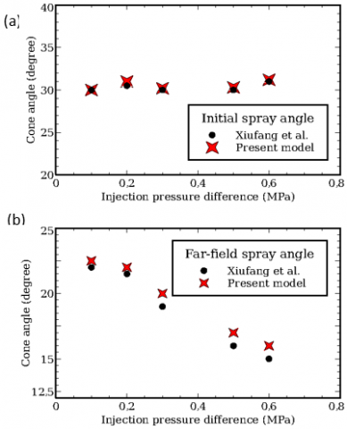
The second comparison is presented in Figure 3, where the aim of the study of atomization by numerical simulation is also needed, for this type of flow, as a complement to the experimental studies. Indeed, this one can allow, on the one hand, to understand more finely the physical phenomena at the initial stages that are difficult to capture in the experimental work in the free flow which is interested in this paper. On the other hand, to characterize the impact of the primary zone of atomization on the whole of the spray. Figure 3a shows the liquid volume fraction at the initial stage of spray atomization. As mentioned in the work of Liu et al. [7], the spray cone angle at (a)initial spray cone angle and (b) far-field spray cone angle. The shape of spray edges near the injector tends to be rounded which is compatible with their sketches. Figure 3b shows the structure of spray taken from Liu et al. [7]. The two structures are approximately the same but it should be followed by another parameter to cutting edge. Unfortunately, experimental data does not exist to demonstrate this. However, the figure has been used to explain the boundaries and the outer edges of the spray. This figure also illustrates the start of the injection period where the liquid seems to be non-uniform which is matching the schematic Figure 3(a) where the experimental cannot capture this phenomenon. Figure 4a shows a comparison between the experimental data extracted from Liu et al. [7] and the presented work for the initial stages of the spray injection at different injection pressures. An excellent agreement is found between the two curves due to taking the same injection and physical parameters for the spray liquid nitrogen.
Figure 4. Comparison between calculated and measured [6] initial spray cone angle at different injection pressure (a) initial spray angle and (b) far-field spray angle
In general, the spray from the nozzle is a cone of a circular section. The angle of injection of this spray corresponds to the opening angle of the cone. It’s a variable that contributes greatly to the spatial dispersion of droplets in the air. The more the angle of a spray is large, the more dispersion of the droplets in the air. The injection angle is not the only parameter governing spatial dispersion droplets. The speed and size of the droplets also play an important role. From Figure 4b and the above illustration is for the initial injection period whereas the spray cone angle tends to decrease far from the injector when the injection pressure is increasing. The purpose of calculating the drop size distribution of different injection pressure sprays is to know the spray characteristics of this type of sprays and compare them to those produced by standard injectors.
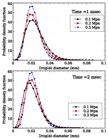
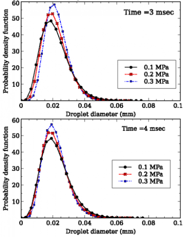
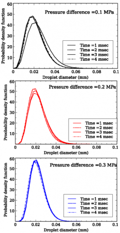
The influence of external parameters on the atomizing qualities of a solid cone injector is also an essential point for understanding the phenomenological direct injection of liquid nitrogen at different injection pressure. The effect of the pressure increases on the size of the droplets formed is examined. Figure 5 shows the probability density function with droplet sizes at different times. For a back pressure of 1 bar and an injection pressure differences ranging between 0.1, 0.2 and 0.3 MPa. Considering problems of repeatability, and therefore of representativity, at 1, 2 and 3 msec, it can be seen that the rise in the probability density function causes a tightening of the drop size distribution accompanied by a slight shift towards small drops. The injection velocity can be estimated from Bernoulli’s theorem, adding a corrective factor called the discharge coefficient, which allows taking into account any pressure losses in the nozzle.
Figure 5. Comparison between probability density function at different injection pressures
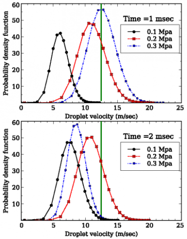
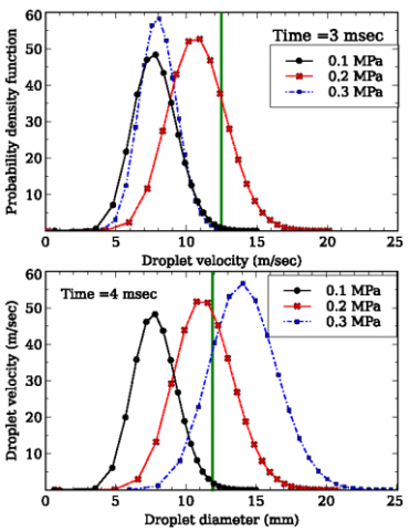
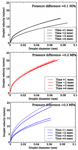
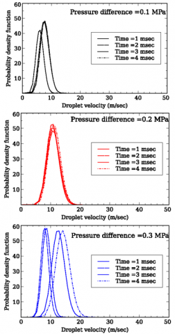
Figure 6 shows the droplet velocity profile at different injection pressures and times. A high-velocity value in the center of the spray that is consistent with that expected for full cone injectors. The maximum velocity is therefore at the center. Then after an increase in injection pressure (over 50%), a much smaller droplet can be found at the periphery, typical of a swirling movement. This is associated with small velocity. Then droplet velocity and its deviation decrease on the extreme edge of the spray. Figure 7 shows the probability density function with a droplet velocity of different injection pressure at different times. The prediction starts with a derivation of the momentum equation. It can be obtained that an estimate of the velocity of moving droplets. The higher probability density function refers to the smaller droplet sizes. It can then be used to estimate the value of the Weber number of spray if the diameter of the droplets is known. At time 1msec most of the spray droplets are having approximately a wide distribution due to the full atomization assumption for all injection pressure cases. At time 2 and 3msec, the distribution of droplets begins to less wide and appears clearly when the different injection pressure is 0.3 MPa. This is because most of the droplets are experienced in the air drag force resistance. At time 4msec the distribution becomes wider due to the increase in the mass flow rate and increase of disintegration processes. Moreover, if the case at 0.3 MPa is excluded, it is found that the trends are developed gradually to each other.
Figure 6. Comparison between droplet velocity at different injection pressures
Figure 7. Comparison between calculated probability density function at different times and injection pressures
It means that the deceleration is the same in all conditions and that the velocity of droplets at the head of the spray at a time given depends only on the initial injection velocity. The atomization of a spray leads to various drop diameters. The sprays obtained are generally very polydispersed. Most atomizers generate drops of diameters ranging from a few microns up to about 500 microns. For that to characterize a spray, in addition to the average drop size, the distribution of the sizes of drops in the spray is another important parameter.
This size distribution of drops is usually represented by histograms or functions of distribution that can be expressed in a number of drops, surface or volume. Each representation depends on the experimental technique or modeling used.
Figure 8. Time evolution of probability density function due to atomization at different injection
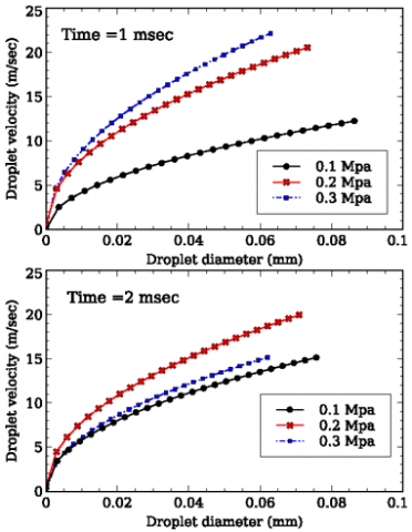
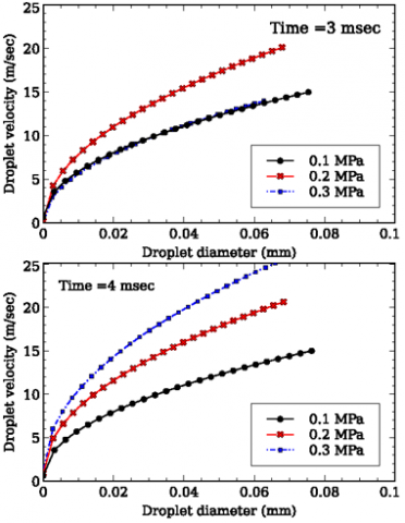
There are different ways to express a representative diameter of the spray studied. The drop size distribution at a different time is generally used. Figure 8 shows the unsteady distribution of drops at different times and different injection pressures. In all cases when the time has proceeded, the probability density function is increased. This makes it possible to characterize globally a spray. To better understand the dynamics of the droplets, it is interesting to complete the information contained in global size and velocity distributions by a study of combined size/velocity distributions. That is to say, the study of sizes and velocity one against the other. Indeed, droplets of very different sizes are present in the spray (from 100 μm to several millimeters) and these droplets may have very different since the way these will respond to the flow of air and their size. But the distributions calculated on the whole of the spray do not allow to identify the respective contribution of different populations of droplets. As examples will be represented in the following distributions droplet velocity profile with droplet diameter, at different times at different injection pressures as shown in Figure 9. The bigger droplets have a higher velocity than others and increased gradually as the droplet diameter increased. Normally, the droplet velocity is increased with injection pressure and with time. As be noticed in all cases, the predicted profile at (4msec) has the highest values due to the atomization processes such as breakup and collision. It should be noted that the droplet velocity profile does not represent the core of the spray where the maximum velocity is found. The drop size distributions of the droplets obtained by atomization processes are very dependent on the operating conditions.
Figure 9. Time evolution of droplet velocity due to atomization at different injection pressures
The relatively high number of studies described in the literature to better understand the relationships between operating parameters and drop size distributions. This issue is important in the atomization of cryogenic fluid. Figure 10 shows the drop size distribution versus droplet velocity of a nitrogen liquid spray under different operating conditions (injection pressure and time). The influence of the injection pressure of the liquid on the shape of the drop size distributions with droplet velocities seems more obvious at pressure difference equal 0.3MPa. For this point, an increase in the flow of nitrogen injected into the nozzle leads to a higher value of the most likely velocity. This is probably due to the height of a greater liquid mass flow rate and therefore increases its average velocity.
On the other hand, it does not distinguish any noticeable difference between the respective values of the most probable velocity of pressure difference 0.2MPa, whereas, for the latter, the drop size distribution height of the spray droplet is less than the other two cases. The injected liquid flow should, therefore, be slower and this trend is observed for droplet velocity. This is probably due to that they are generally larger for pressure difference 0.3MPa and 0.2MPa, and therefore tend to move more quickly.
Figure 10. Time evolution of variation of probability density function with droplet velocity at different injection pressures
A liquid nitrogen spray model that captures the initial and complete hydrodynamics nature of cryogenic sprays without using tracking droplets but by using the maximum entropy method of the droplet size distributions has been applied to solidcone pressure swirl nozzles and liquid nitrogen sprays. The simulated test cases presented in this work indicate that the new cryogenic spray model can be applied to wide cone-angle, high droplet density, and low injection velocity spray cases. The performance of the probability density function has been assessed, and the good prediction of the initial spray cone angle values near the injector indicates that the atomization models perform reasonably. The model fairly captures the spray drop size distribution and the whole structure of the spray when the model uses liquid volume fraction. Though, with an increase in spray injection pressure, the values are in agreement with the experimental image. However, several of points still essential to be improved in the model. The atomization and heat and mass transfer models need to be re-assessed, perhaps other models have to be applied for the cryogenic sprays need to be implemented.
The advantages of the maximum entropy method are, the maximum statistical entropy model obtains the model with the highest entropy of knowledge for all the models that satisfy the constraint conditions. Transport equations need not be solved for the conservation of quantity, momentum and energy. The distribution of entropy can be carefully adjusted in such a way that the most unbiased and optimal distribution model can be obtained. The maximum entropy approach is that it does not require any assumptions about the form of the proposed continuous distribution function while in Lagrangian approach it depends on the number of parcels. Other drop size distribution functions can be used since different types of injectors produce different classes of droplet size distributions. The set of maximum entropy equations is iteratively solved numerically using the Newton-Raphson method to predict unknown Lagrangian multipliers. The equations and derivatives are an integral and exponential equation leads to convergence difficulties in the computational solution. These solutions are highly sensitive to the initial values of Lagrange multipliers. Reasonable initial guesses for the unknown Lagrangian multipliers can lead to faster convergence. The accuracy of using Lagrangian approach in polydispersed phase is always accurately less than Eulerian approach because it depends on the number of parcels while in Eulerian approach it depends on the proposed continuous distribution function. Further work has to be carried out in this area when in this case the different distribution functions are implemented for the results of the droplet drag and breakup processes. Current liquid nitrogen solid-cone pressure injectors can realize injection pressure values of up to 0.6MPa, thus it will be relevant to apply this model to such cases. There are a number of aspects of the mass and heat transfer sub-models that require further investigation in the context of the spray cooling and the distribution of vapour mass flux.
[1] Abbasi, B., Kim, J. (2011). Prediction of PF-5060 spray cooling heat transfer and critical heat flux. Journal of Heat Transfer, 133(10): 101504. https://doi.org/10.1115/1.4004012
[2] Zhang, X.B., Qiu, L.M., Gao, Y., Zhang, X.J. (2008). Computational fluid dynamic study on cavitation in liquid nitrogen. Cryogenics, 48(9-10): 432-438. https://doi.org/10.1016/j.cryogenics.2008.05.007
[3] Ishimoto, J. (2009). Numerical study of cryogenic micro-slush particle production using a two-fluid nozzle. Cryogenics, 49(1): 39-50. https://doi.org/10.1016/j.cryogenics.2008.10.004
[4] Zhang, P., Xu, G.H., Fu, X., Li, C.R. (2011). Confined jet impingement of liquid nitrogen onto different heat transfer surfaces. Cryogenics, 51(6): 300-308. https://doi.org/10.1016/j.cryogenics.2010.06.018
[5] Ishimoto, J., Oh, U., Tan, D. (2012). Integrated computational study of ultra-high heat flux cooling using cryogenic micro-solid nitrogen spray. Cryogenics, 52(10): 505-517. https://doi.org/10.1016/j.cryogenics.2012.07.002
[6] Somasundaram, S., Tay, A.A.O. (2014). A study of intermittent liquid nitrogen sprays. Applied Thermal Engineering, 69(1-2): 199-207. https://doi.org/10.1016/j.applthermaleng.2013.11.066
[7] Liu, X.F., Xue, R., Ruan, Y.X., Chen, L., Zhang, X.Q., Hou, Y. (2017). Effects of injection pressure difference on droplet size distribution and spray cone angle in spray cooling of liquid nitrogen. Cryogenics, 83: 57-63. https://doi.org/10.1016/j.cryogenics.2017.01.011
[8] Liu, X.F., Xue, R., Ruan, Y.X., Chen, L., Zhang, X.Q., Hou, Y. (2017). Flow characteristics of liquid nitrogen through solid-cone pressure swirl nozzles. Applied Thermal Engineering, 110: 290-297. https://doi.org/10.1016/j.applthermaleng.2016.08.150
[9] Xue, R., Ruan, Y., Liu, X., Cao, F., Hou, Y. (2017). The influence of cavitation on the flow characteristics of liquid nitrogen through spray nozzles: A CFD study. Cryogenics, 86: 42-56. https://doi.org/10.1016/j.cryogenics.2017.07.003
[10] Xue, R., Ruan, Y., Liu, X., Chen, L., Hou, Y. (2018). Numerical study of liquid nitrogen cavitating flow through nozzles of various shapes. Cryogenics, 94: 62-78. https://doi.org/10.1016/j.cryogenics.2018.07.009
[11] Xue, R., Chen, L., Zhong, X., Liu, X., Chen, S., Hou, Y. (2019). Unsteady cavitation of liquid nitrogen flow in spray nozzles under fluctuating conditions. Cryogenics, 97: 144-148. https://doi.org/10.1016/j.cryogenics.2018.09.010
[12] Zhang, S., Li, X., Zhu, Z. (2018). Numerical simulation of cryogenic cavitating flow by an extended transport-based cavitation model with thermal effects. Cryogenics, 92: 98-104. https://doi.org/10.1016/j.cryogenics.2018.04.008
[13] Li, L., Xie, M., Wei, W., Jia, M., Liu, H. (2018). Numerical investigation on cryogenic liquid jet under transcritical and supercritical conditions. Cryogenics, 89: 16-28. https://doi.org/10.1016/j.cryogenics.2017.10.021
[14] Xue, R., Ruan, Y., Liu, X., Chen, L., Zhang, X., Hou, Y., Chen, S. (2018). Experimental study of liquid nitrogen spray characteristics in atmospheric environment. Applied Thermal Engineering, 142: 717-722. https://doi.org/10.1016/j.applthermaleng.2018.07.056
[15] Xue, R., Ruan, Y., Liu, X., Chen, L., Liu, L., Hou, Y. (2019). Numerical study of the effects of injection fluctuations on liquid nitrogen spray cooling. Processes, 7(9): 564. https://doi.org/10.3390/pr7090564
[16] Wang, C., Song, Y., Jiang, P.X. (2018). Modelling of liquid nitrogen spray cooling in an electronic equipment cabin under low pressure. Applied Thermal Engineering, 136: 319-326. https://doi.org/10.1016/j.applthermaleng.2018.02.095
[17] Ruan, Y.X., Hou, Y., Xue, R., Luo, G.Q., Zhu, K.Z., Liu, X.F., Chen, L. (2019). Effects of operational parameters on liquid nitrogen spray cooling. Applied Thermal Engineering, 146: 85-91. https://doi.org/10.1016/j.applthermaleng.2018.09.098
[18] Sellens, R.W., Brzustowski, T.A. (1985). A prediction of the drop size distribution in a spray from first principles. Atomization and Spray Technology, 1: 89-102.
[19] Cao, J.M. (2002). On the theoretical prediction of fuel droplet size distribution in nonreactive diesel sprays. Journal of Fluids Engineering, 124(1): 182-185. https://doi.org/10.1115/1.1445140
[20] Dumouchel, C. (2006). A new formulation of the maximum entropy formalism to model liquid spray drop‐size distribution. Particle & Particle Systems Characterization, 23(6): 468-479. https://doi.org/10.1002/ppsc.200500989
[21] Li, X., Tankin, R.S. (1987). Droplet size distribution: a derivation of a nukiyama-tanasawa type distribution function. Comb. Science and Technology, 56: 65-76. https://doi.org/10.1080/00102208708947081
[22] Lecompte, M., Dumouchel, C. (2008). On the capability of the generalized gamma function to represent spray drop-size distribution. Particle & Particle Systems Characterization, 25(2): 154-167. https://doi.org/10.1002/ppsc.200701098
[23] Beck, J.C., Watkins, A.P. (2003). On the development of a spray model based on drop-size moments. Proceedings of the Royal Society of London. Series A: Mathematical, Physical and Engineering Sciences, 459(2034): 1365-1394. https://doi.org/10.1098/rspa.2002.1052
[24] Nmira, F., Kaiss, A., Consalvi, J.L., Porterie, B. (2008). Predicting fire suppression efficiency using polydisperse water sprays. Numerical Heat Transfer, Part A, 53: 132-156. https://doi.org/10.1080/10407780701453669
[25] Carneiro, J.N., Kaufmann, V., Polifke, W. (2009). Numerical simulation of droplet dispersion and evaporation with a moments-based CFD model. In Proceeding of 20th International Congress of Mechanical Engineering, pp. 15-20.
[26] Laurent, C., Lavergne, G., Villedieu, P. (2010). Quadrature method of moments for modeling multi-component spray vaporization. International Journal of Multiphase Flow, 36(1): 51-59. https://doi.org/10.1016/j.ijmultiphaseflow.2009.08.005
[27] Hosseinalipour, S.M., Karimaei, H., Movahednejad, E. (2016). Droplets diameter distribution using maximum entropy formulation combined with a new energy-based sub-model. Chinese Journal of Chemical Engineering, 24(11): 1625-1630. https://doi.org/10.1016/j.cjche.2016.03.004
[28] Shannon, C.E. (1948). A mathematical theory of communications. The Bell System Technical Journal, 27(3): 379-623. https://doi.org/10.1002/j.1538-7305.1948.tb01338.x
[29] Reitz, R. (1987). Modeling atomization processes in high-pressure vaporizing sprays. Atomisation and Spray Technology, 3(4): 309-337.
[30] Wallis, G.B. (1969). One-Dimensional Two-Phase Flow. McGrawHill, New York.
[31] O'Rourke, P.J. (1981). Collective Drop Effects on Vaporizing Liquid Sprays (No. LA-9069-T). Los Alamos National Lab., NM (USA).
[32] Majhool, A.A.A.K. (2011). Advanced spray and combustion modelling. Doctoral dissertation, the University of Manchester, United Kingdom.
[33] Spalding, D.B. (1953). The combustion of liquid fuels. Symposium (International) on Combustion, 4(1): 847-864. https://doi.org/10.1016/S0082-0784(53)80110-4
[34] Samareh, B., Dolatabadi, A. (2008). Dense particulate flow in a cold gas dynamic spray system. Journal of Fluids Engineering, 130(8): 081702. https://doi.org/10.1115/1.2957914
[35] Launder, B.E., Spalding, D.B. (1972). Lectures in Mathematical Models of Turbulence. Academic Press, London, England.
[36] Launder, B.E., Sharma, B.I. (1974). Application of the energy-dissipation model of turbulence to the calculation of flow near a spinning disc. Letters in Heat and Mass Transfer, 1(2): 131-137. https://doi.org/10.1016/0094-4548(74)90150-7