Elena Campagnoli* | Valter Giaretto
© 2020 IIETA. This article is published by IIETA and is licensed under the CC BY 4.0 license (http://creativecommons.org/licenses/by/4.0/).
OPEN ACCESS
From a thermal point of view, water-agar gel can reproduce the behavior of human soft tissues with a good approximation. For this reason, agar gel is widely used to mimic the thermal diffusion inside the latter, in order to study the effect on human tissues of new techniques and probes used to solve various health diseases. Cryoablation is part of these techniques and its effectiveness strongly depends on the biological response of the tissues to the freezing action and heat diffusion and therefore on their thermo-physical properties. This study presents the values of thermal conductivity and thermal diffusivity, measured on water-agar gel samples, using the transient plane source method, forward and backward from room temperature down to -60℃. The freezing transient and the temperature at which the phase transition begins are highlighted, as well as the temperature dependence of both thermal conductivity and diffusivity.
water-agar gel, experimental investigation, thermal conductivity, thermal diffusivity, cryoablation
Agar is a substance (unbranched polysaccharide) extracted from several species of red seaweeds, which has many applications in different fields.
For example, agar is used to prepare foods and beverages for people suffering from celiac disease who need a gluten free diet [1, 2]. Several studies report information on seaweeds-based composites used for food packaging as well as for pharmaceutical applications [3, 4].
Agar also plays a crucial role in medicine, where it is used as tissue-mimicking phantom because it reproduces the thermal behavior of biological soft tissues with a good approximation. For this reason, agar can be a good substitute for ex vivo animal tissues, for example bovine tissues (e.g. liver and heart), commonly used in experimental investigations [5, 6]. Based on what just written, the agar gel could be used to better understand the behavior of the biological tissues when the latter undergo a process of cryoablation.
Today cryoablation is a procedure used in various medical therapies on patients suffering for example from cancer or atrial fibrillation [7-9] and a deep knowledge of the tissues response to this freezing could increase the success rate by reducing recurrences. The cooling dynamics (i.e. the temperature at which the formation of ice begins and the rate at which it advances) depends on the equipment available and on other parameters such as the temperature of the freezing agent and the cooling rate. These last two parameters are strictly connected to the behavior of the tissues and therefore to their thermo-physical properties.
As far as the authors know, the thermal properties of the agar gel at low temperature are not reported in the literature. The only paper found in the literature [10] shows the effect of agar concentration on the thermal conductivity of water–agar gel samples at temperatures well above the freezing point.
For this reason, the purpose of this work was to investigate the temperature dependence of the thermal conductivity, and thermal diffusivity of water-agar gel samples from room temperature down to -60℃. The experiments were carried out using the transient plane source method, which is commonly applied to measure the thermal conductivity of liquids, foams and solids in the range 0.1 ÷ 100 Wm-1K-1 [11-13].
In the paper are described the method and the apparatus used to carry out the experimental investigation, as well as the procedure used to prepare the samples. The results obtained are shown and discussed.
The device used to perform the measurements is a commercial instrument, a Hot Disk® model TPS 500. This instrument applies the transient plane source method to measure the thermal conductivity and thermal diffusivity of solid materials while allowing the calculation of the volumetric specific heat [14, 15].
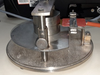
The TPS 500 uses a sensor that works at the same time as heat source and thermometer. The sensor (Figure 1) consists of a very thin metallic double spiral (concentric rings), sealed between two Kapton sheets, which act as electrical insulators.
The sensor has four electrical connections: two of them carry the heating current while the other two are used as a resistance thermometer, which measures the voltage drop across the spiral.
The experiments are performed applying a stepwise current to a C5501 sensor [16], 6.403 mm in radius and with 14 concentric rings, which is clamped between two samples of the material to be tested (Figure 1). In this way, a Joule heating is obtained, which produces a temperature transient in both the sample and the sensor.
The dependence on the temperature of the electrical resistance of the sensor is determined, according to Eq. (1):
$R(t)=R_{0} \cdot\left[1+\beta \cdot \Delta T_{S}(t)\right]$ (1)
In Eq. (1) the average temperature increase DTS(t), at each time t, is determined using the value of the reference resistance R0 and the temperature coefficient b. These last two parameters are obtained by calibration performed by the manufacturer.
Figure 1. Typical assembly of samples and sensor
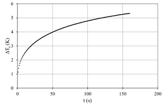
An example of the increase in the average sensor temperature recorded is shown in Figure 2 as a function of time. In the post process phase, the apparatus analyses this temperature transient to measure both the thermal diffusivity and the thermal conductivity of the material under test.
Figure 2. Average increase in sensor temperature vs time
Neglecting the initial part of the transient (usually less than a couple of seconds and due to the insulation of the sensor), the measured average temperature increase is in good agreement with
$\Delta T_{s}(\tau)=m \cdot F(\tau, n)$ (2)
where, m is a parameter, which will be discussed after, and $F(\tau, n)$ a shape function, for the number n of concentric rings of the heat source, which depends on the dimensionless time $\tau$ as shown in the following equation
$F(\tau, n)$$=[n \cdot[n+1]]^{-2} \int_{0}^{\tau} \varepsilon^{-2}\left[\sum_{i=1}^{n} i \sum_{j=1}^{n} j \exp \left(-\frac{i^{2}+j^{2}}{4 n^{2} \varepsilon^{2}}\right) \cdot I_{0}\left(\frac{i \cdot j}{2 n^{2} \varepsilon^{2}}\right)\right] d \varepsilon$ (3)
where, ε is a dummy integration variable, and I0 is the modified Bessel function of the first kind zero order.
With the well-defined number n of concentric rings, the shape function is obtained by integrating the instantaneous ring source over the dimensionless time t [17], which in turn depends on the thermal diffusivity a:
$\tau=\frac{\sqrt{\alpha \cdot t}}{r}$ (4)
Figure 3, for the measured transient reported in Figure 2, shows the linear relationship between $\Delta T_{S}(\tau)$ and $F(\tau, n)$, established by Eq. (2), and allows to determine both the thermal diffusivity and the thermal conductivity of the sample.
Figure 3. Average increase in sensor temperature vs shape function
In fact, the numerical value of the thermal diffusivity $\alpha$ is the one that produces the maximum likelihood for the linear trend imposed by Eq. (2), with the slope m linked to the thermal conductivity $\lambda$ as:
$m=\frac{P}{\pi^{3 / 2} \cdot r \cdot \lambda}$ (5)
where, P is the input power and r is the radius of the sensor.
Using the TPS 500 the declared accuracy for thermal conductivity is ±5%, while the declared reproducibility is ±10% for thermal diffusivity, and ±12 % for volumetric specific heat [16, 18].
4.1 Preliminary tests
Using the reference samples supplied with the TPS, some preliminary tests were carried out, from room temperature to -60℃, to check the behavior of the components of the equipment when they are placed in the CTC during the experiments. The reference samples, shown in Figure 1, are made of steel type SIS2343 (equivalent to AISI 316).
The measured values of thermal conductivity for the reference material versus temperature are shown in Figure 6. The comparisons of the measured values with those of literature [19] showed a good agreement within the accuracy declared for the TPS (error bars ± 5%). This verification has therefore made it possible to verify that there is no reason to consider inappropriate the use of the apparatus inside the CTC within the mentioned temperature range.
Figure 6. Thermal conductivity vs temperature for the steel reference samples (error bar ± 5%)
4.2 Water – agar gel tests
Tests on the agar samples were performed in the above mentioned temperature range. All samples were tested executing measurements back and forth from ambient temperature down to -60℃ and vice versa, fixing in this range some intermediate values useful to identify the temperature trends and the onset of the phase transition.
For each temperature set, the measurements were executed waiting for both the CTC and the sample to reach steady state conditions. The initial set point temperature was chosen lower than the laboratory temperature (about 10℃ lower) to overcome the difficulties of the CTC temperature controller in achieving stability around ambient conditions. At any set point, two consecutive measurements were performed by changing the input thermal power P, in the range 100 mW ÷ 300 mW, or alternatively the duration of the thermal impulse, in the range 40 ÷ 120 s. At each temperature the average values of the measured properties was considered.
Table 1 shows the number of measurements performed on each of the three samples in the different temperature ranges. In Table 1, measurements taken during cooling down to -60℃ and measurements taken during subsequent heating to return to room temperature are classified as forward (F) and backward (B), respectively.
Table 1. Number of measurements performed
|
|
Sample 1 |
Sample 2 |
Sample 3 |
|||
|
T (℃) |
F |
B |
F |
B |
F |
B |
|
-1.9 ÷ 10.9 |
3 |
2 |
3 |
2 |
3 |
2 |
|
Around -3.5 |
- |
- |
2 |
- |
- |
- |
|
-4.9 ÷ -14 |
2 |
1 |
2 |
2 |
2 |
1 |
|
-14 ÷ -61 |
6 |
4 |
7 |
4 |
6 |
4 |
Figure 7 reports, for a set point temperature of -6.3℃, two examples of temperature increase, obtained with an input power of 300 mW and 250 mW respectively, and with a pulse duration of 60 s for both the cases.
Figure 7. Example: sample temperature measured using the thermocouple placed near the outer edge of the sensor
It can be noted that for both the measurements the temperature increase, recorded by the thermocouple at the sensor boundary, is very small and slightly higher than 0.5℃. Furthermore, Figure 7 shows that while the time for the increase in temperature, corresponding to the duration of the pulse is 60 s, the relaxation time, i.e. the time required to return to the initial temperature, is about an order of magnitude higher.
In previous experiments [5], devoted to investigate the formation and growth of ice inside the agar gel, during which a cooling rate of about 20 K/min was used, the beginning of the formation of ice was found in a super-cooled state at temperatures around -7℃.
In the present experiments, with very low cooling rates (more than two orders of magnitude smaller than the previous one), the onset of the phase transition was expected at higher temperature, closer to the triple point of pure water. Therefore, to identify the thermal properties as close as possible to the onset of the phase transition, several measurements were carried out in the temperature range between the triple point of water and the onset temperature of ice formation reported in the reference [5].
Figure 8. Onset of the phase transition and set of measurements to identify the properties of water – agar
The typical behavior observed at the onset and during the phase transition is reported in Figure 8 as an example. Initial ice formation was clearly detected for all samples with a sudden increase in temperature, from the onset value (-3.5℃ in the case shown in Figure 8) to a value just under the triple point of pure water (-0.2℃ in Figure 8).
After this sudden increase in temperature, the phase transition occurs in the entire volume of the sample with a slow isothermal process. In the tested samples, some differences were observed in the temperature of the onset of the phase change, with values between -2.5℃ and -4.2℃. When the transition is completed, the temperature begins to decrease slowly and the sample reaches the reference value at which it is desired to determine the properties, represented in this case by the state A, -6.3℃ (Figure 8).
For the case shown in Figure 8, attempts were made to measure the properties of the water–agar gel during the phase transition, state A’, and along the transient toward the reference temperature, state A”. Both attempts highlighted critical issues in determining properties.
Regarding state A’, the heat released due to the phase change overlaps with that generated by Joule effect through the hot disk, disturbing the measurement signal and preventing any determination of the properties regardless of the input thermal power adopted.
A different kind of analysis must be done for the measurement at the state A” (Figure 8), carried out during the cooling phase. Despite the slow rate of cooling (about 0.04 K/min), the determination of the properties under transient conditions involves a bias in the calculated residuals, i.e. a lack of linearity in the shape function mentioned above respect to the temperature increase measured (see Figure 3), which provides a lower reliability of the measured value. Nonetheless, these measurements were initially considered in the analysis with the same precision as the others.
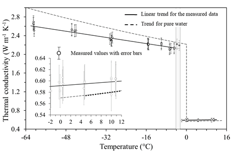
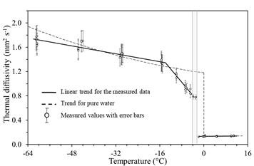
For all the agar samples tested, the measured values of the thermal conductivity and thermal diffusivity as a function of the temperature are shown in Figures 9 and 10 respectively.
Figure 9. Thermal conductivity vs temperature
Figure 10. Thermal diffusivity vs temperature
Table 2. Linear regression coefficients (T0 = 273.15 K)
|
Thermal properties |
Coefficients |
|
Conductivity, $\mathrm{W} /(\mathrm{m} \mathrm{K})$ |
$-1.9^{\circ} \mathrm{C} \leq\left(T-T_{0}\right) \leq 10.9^{\circ} \mathrm{C}$ $a_{\lambda}=0.5917 \mathrm{W} /(\mathrm{m} \mathrm{K})$ $b_{\lambda}=0.0011\left(\mathrm{K}^{-1}\right)$ $-61^{\circ} \mathrm{C} \leq\left(T-T_{0}\right) \leq-4.9^{\circ} \mathrm{C}$ $a_{\lambda}=2.0987 \mathrm{W} /(\mathrm{m} \mathrm{K})$ $b_{\lambda}=-0.0039\left(\mathrm{K}^{-1}\right)$ |
|
Diffusivity, $\mathrm{mm}^{2} / \mathrm{s}$ $\alpha(T)=a_{\alpha}\left[1+b_{\alpha}\left(T-T_{0}\right)\right]$ |
$\begin{aligned}-1.9^{\circ} \mathrm{C} & \leq\left(T-T_{0}\right) \leq 10.9^{\circ} \mathrm{C} \\ a_{\alpha} &=0.1342 \mathrm{mm}^{2} / \mathrm{s} \\ b_{\alpha} &=0.0035\left(\mathrm{K}^{-1}\right) \\-14^{\circ} \mathrm{C} & \leq\left(T-T_{0}\right) \leq-4.9^{\circ} \mathrm{C} \\ a_{\alpha} &=0.5902 \mathrm{mm}^{2} / \mathrm{s} \end{aligned}$ $\begin{aligned} b_{\alpha} &=-0.0918\left(\mathrm{K}^{-1}\right) \\-61^{\circ} \mathrm{C} & \leq\left(T-T_{0}\right) \leq-14^{\circ} \mathrm{C} \\ a_{\alpha} &=1.2320 \mathrm{mm}^{2} / \mathrm{s} \\ b_{\alpha} &=-0.0066\left(\mathrm{K}^{-1}\right) \end{aligned}$ |
|
Volumetric specific heat, $\mathrm{MJ} /\left(\mathrm{m}^{3} \mathrm{K}\right)$ |
$\rho c(T)=\frac{a_{\lambda}\left[1+b_{\lambda}\left(T-T_{0}\right)\right]}{a_{\alpha}\left[1+b_{\alpha}\left(T-T_{0}\right)\right]}$ |
The investigation was performed moving back and forth within the specified temperature range, imposing for each sample a freeze – thaw thermal cycle, starting from room temperature and returning to it. Referring to the measurement accuracy and repeatability declared for the TPS 500 apparatus, no hysteresis of the measured properties along the freeze – thaw cycle was identified for any sample.
In these figures, the vertical gray bar represents the temperature range (-2.5℃ ¸ -4.2℃) in which the onset of ice formation was detected in the cooling processes performed. In Figure 9 and Figure 10 the empty and black circles represent the measurements performed. The error bars are ±5% and ±10% respectively for thermal conductivity and thermal diffusivity, showing a good repeatability of all the measurements, independently of the possible inhomogeneity of the samples. The black circles inside the gray band refer to the measurements carried out in the state A” of Figure 8. Solid lines are the best linear fits of the property values obtained for frozen and non-frozen states. In the case of thermal diffusivity (Figure 10), two linear trends were assumed for measurements in the frozen state before and after -14℃. Linear regression coefficients are reported in Table 2 for both the measured properties.
In the temperature range -1.9℃ ¸ -4.9℃ it was not possible to perform measurements at steady state. Assuming for the properties determined in this range (state A”) the same measurement precision used for the other points (steady state), and linking these values with the trends calculated for the frozen state, it was clear that these data could not be excluded from the statistics, as shown in Figure 9 and Figure 10.
Comparing (Figures 9 and Figure 10) the linear trends calculated for both the thermal conductivity and diffusivity (solid lines) with the values found in literature [20] for pure water (dashed lines), a similar behavior clearly appears for the states at a temperature above the freezing point. On the contrary, considerable differences can be noted for the values after freezing. An attempt was also made to compare the obtained thermal conductivity with literature data for mixtures of water and agar at different concentrations [10].
Unfortunately, in the temperature range of validity for these experimental results (greater than 5℃), with the concentration of agar at 2%, the thermal conductivity values are practically coincident with those of pure water.
Considering the measured values with the relative error bars, there are no significant differences, neither for the thermal conductivity nor for the thermal diffusivity, between the samples made of water – agar gel investigated and the pure water above its triple point, on the contrary appreciable differences were found in the frozen state.
After the onset of the phase transition, and then at lower temperatures, the thermal conductivity of agar gel shows a trend similar to that of pure water albeit with appreciably lower values, while for the thermal diffusivity the most evident differences with water concern what happens immediately after the phase transition. This behavior of agar gel was highlighted introducing two different slopes for the linear trends of the thermal diffusivity versus temperature, as shown in Figure 10. To try to provide a plausible explanation for this behavior, a preliminary investigation was performed on the structure of the water - agar mixture, before and after the phase change.
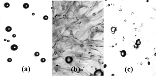
The micrographs in Figure 11, made with a transmission microscope with 25´ magnification, show the water – agar structure before freezing (a), when frozen (b) and after thawing (c). Pictures (a) and (c) were taken at the room temperature, while picture (b) was taken at a temperature close to that at which in the frozen state the trend of the thermal diffusivity versus temperature changes.
Each sample shows air bubbles trapped in the gel of a few tenth of millimeter. The presence of air bubbles and their size are in agreement with what is reported in the literature [21].
Samples in picture (a) and (c) show a similar structure for the water-agar gel matrix, and this fact can probably justify the absence of hysteresis phenomena in the measured thermal properties, during the freeze-thaw cycles.
Before the ice formation, picture (a), the structure appears homogeneous with agar powder well dispersed in the water. After the phase transition the structure is clearly different. In fact, sample in picture (b), which shows the growth of ice within the matrix of agar, exhibits an uneven structure with disordered ice crystals. This occurrence can probably explain the reduced conductivity of the frozen agar gel in comparison with pure water. Furthermore, the scattered growth of ice is probably also responsible for a different dependence of the density on the temperature, and it could justify the less abrupt transition in the measured values of thermal diffusivity.
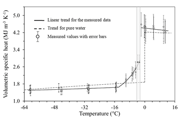
The volumetric specific heat $\rho c(T)$ shown in Figure 12 was obtained from the definition of thermal diffusivity, using the equations and coefficients in Table 2. This diagram is consistent with the previous analysis, and the continuous line, obtained using the aforementioned analytical relations, is in good agreement with the values calculated starting from the measured thermal conductivity and diffusivity values.
Figure 11. Samples structure: before (a) and during freezing (b) and after thawing (c). Area of the samples 2´3 mm2
Figure 12. Volumetric specific heat vs temperature
The stimulus in characterizing the thermal properties of the water – agar gel in the specified temperature range arises from laboratory needs involving the authors, or more generally, researchers interested in the heat diffusion, ice formation and its growth inside biological tissues. As mentioned in the introduction section, to try to make the cryoablation treatments more effective it is necessary to reproduce in laboratory and to model the thermal effects induced by a cryoprobe on the involved biological tissues employing, at the beginning, materials that allow mimicking their behavior.
Linear temperature dependent functions were experimentally obtained for the heat diffusion properties of the water -agar gel (thermal conductivity and diffusivity) before and after the phase transition (see Table 2), whereas the inspection on the ice onset and its heat of formation goes beyond the scope of this paper.
The limited literature on thermal properties of the water-agar gel, in particular in the temperature range investigated, makes it impossible to give adequate emphasis to the obtained results by comparing them with those of others authors. However, some concluding remarks can be summarized as follows:
|
a, b |
Regression coefficients |
|
|
c |
Specific heat, J. kg-1. K-1 |
|
|
CTC |
Climatic Test Chamber |
|
|
F |
Dimensionless shape function |
|
|
I0 |
Modified Bessel function |
|
|
m |
Parameter (slope) in Eq. (2) and Eq. (5), K |
|
|
n |
Number of concentric rings of the heat source |
|
|
P |
Input power, W |
|
|
r |
Radius of the sensor, m |
|
|
R |
Sensor resistance, W |
|
|
rc |
Volumetric specific heat, MJ. m-3. K-1 |
|
|
T |
Temperature, K |
|
|
t TPS |
Time, s Transient Plane Source |
|
|
Greek symbols |
||
|
$\alpha$ |
Thermal diffusivity, m2. s-1 |
|
|
$\beta$ |
Temperature coefficient of the sensor resistance, K-1 |
|
|
$\varepsilon$ |
Dummy integration variable |
|
|
$\Delta \mathrm{T}_{\mathrm{S}}$ |
Measured temperature increment, K |
|
|
$\lambda$ |
Thermal conductivity, W. m-1. K-1 |
|
|
$\rho$ |
Density, kg. m-3 |
|
|
$\tau$ |
Dimensionless time |
|
[1] Phillips, G.O., Williams, P.A. (2009). Handbook of Hydrocolloids (2nd Edition). Woodhead Publishing. https://doi.org/10.1533/9781845695873
[2] Salehi, F. (2019). Improvement of gluten-free bread and cake properties using natural hydrocolloids: A review. Food Science and Nutrition, 7(11): 3391-3402. https://doi.org/10.1002/fsn3.1245
[3] Khalil, H.P.S.A., Saurabh, C.K., Tye, Y.Y., Lai, T.K., Easa, A.M., Rosamah, E., Fazita, M.R.N., Syakir, M.I., Adnan, A.S., Fizree, H.M., Aprilia, N.A.S., Banerjeee, A. (2017). Seaweed based sustainable films and composites for food and pharmaceutical applications: A review. Renewable and Sustainable Energy Reviews, 77: 353-362. https://doi.org/10.1016/j.rser.2017.04.025
[4] Sousa, A.M.M., Gonçalves, M.P. (2015). Strategies to improve the mechanical strength and water resistance of agar films for food packaging applications. Carbohydrate Polymers, 132: 196-204. https://doi.org/10.1016/j.carbpol.2015.06.022
[5] Giaretto, V., Passerone, C. (2017). Mirror image technique for the thermal analysis in cryoablation: Experimental setup and validation. Cryobiology, 79: 56-64. https://doi.org/10.1016/j.cryobiol.2017.09.001
[6] Giaretto, V., Ballatore, A., Passerone, C., Desalvo, P., Matta, M., Saglietto, A., De Salve, M., Gaita, F., Panella, B., Anselmino, M. (2019). Thermodynamic properties of atrial fibrillation cryoablation: A model-based approach to improve knowledge on energy delivery. Journal of Royal Society Interface, 16(158): 1-8. https://doi.org/10.1098/rsif.2019.0318
[7] Blechinger, J.C., Madsen, E.L., Frank, G.R. (1988). Tissue-mimicking gelatin-agar gels for use in magnetic resonance imaging phantoms. Medical Physics, 15(4): 629-636. https://doi.org/10.1118/1.596219
[8] Adamowicz, J., Tworkiewicz, J., Siekiera, J., Drewa, T. (2013). Ablative therapies for small renal tumors. Contemporary Oncology, 17(1): 24-28. https://doi.org/10.5114/wo.2013.33770
[9] Anselmino, M., D’Ascenzo, F., Amoroso, G., Ferraris, F., Gaita, F. (2012). History of transcatheter atrial fibrillation ablation. Journal of Cardiovascular Medicine, 13(1): 1-8. https://doi.org/10.2459/JCM.0b013e32834ead59
[10] Zhang, M., Che, Z., Chen, J., Zhao, H., Yang, L., Zhong, Z., Lu, J. (2011). Experimental determination of thermal conductivity of water-agar gel at different concentrations and temperatures. Journal of Chemical & Engineering Data, 56(4): 859-864. https://doi.org/10.1021/je100570h
[11] Ai, Q., Hu, Z.W., Wu, L.L., Sun, F.X., Xie, M. (2017). A single-sided method based on transient plane source technique for thermal conductivity measurement of liquids. International Journal of Heat and Mass Transfer, 109: 1181-1190. https://doi.org/10.1016/j.ijheatmasstransfer.2017.03.008
[12] Solorzano, E., Reglero, J.A., Rodriguez-Perez, M.A., Lehmhus, D., Wichmann, M., de Saja, J.A. (2008). An experimental study on the thermal conductivity of aluminium foams by using the transient plane source method. International Journal of Heat and Mass Transfer, 51(25-26): 6259-6267. https://doi.org/10.1016/j.ijheatmasstransfer.2007.11.062
[13] Oaddi, R., Tiskatine, R., Boulaid, M., Bammou, L., Aharoune, A., Ihlal, A. (2019). Thermo-physical properties measurements of an insulating material extracted from different date palm trees. Instrumentation Mesure Métrologie, 18(3): 281-287. https://doi.org/10.18280/i2m.180308
[14] Gustafsson, S.E., Karawacki, E., Khan, M.N. (1979). Transient hot-strip method for simultaneously measuring thermal conductivity and thermal diffusivity of solids and fluids. Journal of Physics D: Applied Physics, 12(9): 1411. https://doi.org/10.1088/0022-3727/12/9/003
[15] Gustafsson, S.E., Ahmed, K., Hamdani, A.J., Maqsood, A. (1982). Transient hot‐strip method for measuring thermal conductivity and specific heat of solids and fluids: Second order theory and approximations for short times. Journal of Applied Physics, 53(9): 6064-6068. https://doi.org/10.1063/1.331557
[16] Hot Disk Thermal Constants Analyser: TPS 500. https://www.hotdiskinstruments.com/products-services/instruments/tps-500/, accessed on 10 July 2020.
[17] Carslaw, H.S., Jaeger, J.C. (1959). Conduction of Heat in Solids. Oxford University Press, p. 260.
[18] Log, T., Gustafsson, S.E. (1995). Transient plane source (TPS) technique for measuring thermal transport properties of building materials. Fire and Materials, 19(1): 43-49. https://doi.org/10.1002/fam.810190107
[19] Bradely, P.E., Radebaugh, R. (2013). Properties of selected material at cryogenics temperatures. CRC Handbook of chemistry and Physics.
[20] Fukusako, S., Yamado, M. (1993). Recent advances in research on water-freezing and ice-melting problems. Experimental Thermal and Fluid Science, 6(1): 90-105. https://doi.org/10.1016/0894-1777(93)90044-J
[21] Ross, K.A., Pyrak-Nolte, L.J., Campanella, O.H. (2006). The effect of mixing conditions on the material properties of an agar gel-microstructural and macrostructural considerations. Food Hydrocolloids, 20(1): 79-87. https://doi.org/10.1016/j.foodhyd.2005.01.007