Jingbin Song* | Lifeng Zheng
© 2020 IIETA. This article is published by IIETA and is licensed under the CC BY 4.0 license (http://creativecommons.org/licenses/by/4.0/).
OPEN ACCESS
To solve problems in the formation mechanism of water flow in automotive water tank and its complex working conditions, this paper constructed a theoretical model for the uncertainty of water jet in automotive water tank. Then, based on the secondary development characteristics of FLUENT software, the uncertainty model, and the fluid field simulation module, this paper studied the wall effect of the fluid field of water jet in automotive water tank, and obtained fluid fields of single-nozzle and double-nozzle water jet and the corresponding distribution laws of the wall effect. The research results showed that the wall effect had a great influence on the direction of the water jet and the pressure on the wall surface of the water tank, while its influence on the velocity of the water jet was relatively small; the two streams of water jet converged, which was basically consistent with the laws of the wall effect in the water tank; the smaller the distance between the two water jet streams, the more likely the two streams would converge. The research in this paper provided theoretical basis and reliable technical support for the analysis of the formation mechanism of the water flow in automotive water tank, the optimization of the water tank structure and the application of water tank in various industries.
automotive water tank, uncertainty model, fluid field, wall effect, numerical simulation
Automotive water tank is one of the important components in the cooling system of automobiles, and the performance of water tank directly determines the performance of the cooling system. To ensure the cooling of the car during actual driving, the water tank must have certain strength and rigidity. To manufacture automotive water tank with excellent comprehensive performance, many scholars at home and abroad have studied the relevant characteristics of the water tank and the water tank bracket. For example, Scholar Asfandiyar et al. [1] polycrystalline SnSe-Sn1-vS solid solutions in vacancy engineering and nanostructuring leading to high thermoelectric performance; O'Connor et al. [2] surgical treatment of tethered cord syndrome in adults for a systematic review and meta-analysis; Cao et al [3] analysis of differential gene expression in response to anisotropic stretch using a systems model of cardiac myocyte mechanotransduction; Li et al. [4] numerical simulation and application of noise for high-power wind turbines with double blades based on large eddy simulation model; Rochling Automotive SE & Co. KG [5] multi-part injection-molded multi-chamber plastic tank having an oblique joining surface in patent application approval process; Iiyama et al [6] a point-estimate based method for soil amplification estimation using high resolution model under uncertainty of stratum boundary geometry; Chandramouli et al. [7] coarse large-eddy simulations in a transitional wake flow with flow models under location uncertainty; Winiarski et al. [8] performance during competition and competition outcome in relation to testosterone and cortisol among women; Fan et al. [9] a review on experimental design for pollutants removal in water treatment with the aid of artificial intelligence; Córcoles-Tendero et al. [10] numerical simulation of the heat transfer process in a corrugated tube; Verkade et al. [11] estimating predictive hydrological uncertainty by dressing deterministic and ensemble forecasts; a comparison, with application to Meuse and Rhine; Kumaran et al. [12] prediction of surface roughness in abrasive water jet machining of CFRP composites using regression analysis; Harless et al. [13] heat transfer and friction characteristics of fully developed gas flow in cross-corrugated tubes; Sydeman et al. [14] best practices for assessing forage fish fisheries-seabird resource competition; Henry et al. [15] performance during competition and competition outcome in relation to testosterone and cortisol among women; Xu et al. [16] study of surface roughness in wire electrochemical micro machining. The above-mentioned scholars have conducted in-depth studies on the various characteristics of the turbines. However, there are few studies concerning the mechanical properties of the automotive water tank under actual working conditions such as strength and stiffness, how the water flows inside the water tank, and the destructiveness of the water flows to the water tank. To this end, this paper took the automotive water tank as the research object, constructed an uncertainty model for the fluid field of the water flow in the automotive water tank, and applied numerical calculation and finite element simulation to study the characteristics of the fluid field in the automotive water tank. This paper aims to provide theoretical basis and technical support for optimizing the water tank structure, designing the positions of the nozzles and improving the service life of the water tank.
According to the principle of the wall surface of the automotive water tank (hereinafter referred to as the water tank), the void ratio near the wall surface of the water tank is larger than that inside the water tank; this is because the resistance of the water tank wall surface is smaller, so the velocity of the flowing water near the tank wall is greater than that inside the water tank. When water jet occurs in the water tank, the water is ejected from the nozzle at a high speed, as the ejected water stream approaches the wall surface of the water tank, the wall effect of the water tank has a certain influence on the flow characteristics of the water, which would further affect the internal structure and service life of the water tank. Therefore, it’s quite necessary to study the fluid field inside the water tank.
The main fluid medium in the water tank is water, and the fluid field in the water tank is mainly shown as the water jet. This paper mainly studied the characteristics of water jet in the water tank.
In the water jet model, it’s assumed that the cylindrical coordinate system of the water jet was (r, θ, z), the radius of the circular nozzle of the water jet was r, the water jet direction was opposite to the direction of z-axis, and the medium around the tank was air, then the equation of the water jet in the water tank was obtained as:
$\left\{\begin{array}{c}\frac{\partial p}{\partial t}+v \cdot \nabla \rho+\rho l v_{r}=0 \\ \frac{\partial v_{r}}{\partial t}+(v \cdot l) v_{r}=-\frac{1}{\rho} \nabla p+u l^{2} v_{r}+\frac{1}{3} u \nabla\left(l \cdot v_{r}\right)\end{array}\right.$ (1)
where, p is the jet pressure; t is the jet time; v is the jet velocity; vr is the disturbance velocity of the water flow; ρ is the water density; $l=\sqrt{\frac{\partial^{2}}{\partial_{r}^{2}}+\frac{1}{r} \cdot \frac{\partial}{\partial_{r}}+\frac{1}{r^{2}} \cdot \frac{\partial^{2}}{\partial \theta^{2}}+\frac{\partial^{2}}{\partial_{z}^{2}}}$ is an intermediate constant variable; u is viscosity coefficient of the motion of the water.
In case of water fluid medium, the relationship between the water jet pressure, the water density and the propagation velocity of sound in water is:
$\frac{\partial p}{\partial \rho}=c^{2}$ (2)
where, c is the propagation velocity of sound in water.
According to the simultaneous Eqns. (1) and (2), the equation of the water jet in the water tank can be obtained as:
$\left\{\begin{array}{r}l \cdot v_{r}+\frac{1}{\rho c^{2}}\left(\frac{\partial p}{\partial t}-v \frac{\partial p}{\partial z}\right)=0 \\ \frac{\partial v_{r}}{\partial t}-v \frac{\partial v_{r}}{\partial z}+\frac{1}{\rho}\left[1+\frac{u}{3 c^{2}}\left(\frac{\partial}{\partial t}-v \frac{\partial}{\partial z}\right)\right] \nabla p=u l^{2} v_{r}\end{array}\right.$ (3)
According to Eq. (3) and the flow characteristics of the fluid, the equation of the liquid water jet of the fluid medium can be obtained as:
$\left\{\begin{array}{c}l \cdot v_{r}+M_{a}^{2}\left(\frac{\partial p}{\partial t}-\frac{\partial p}{\partial z}\right)=0 \\ \frac{\partial v_{r}}{\partial t}-\frac{\partial v_{r}}{\partial z}+\left[1+\frac{M_{a}^{2}}{3 R_{e}}\left(\frac{\partial}{\partial t}-\frac{\partial}{\partial z}\right)\right] \nabla p=\frac{1}{R_{e}} l^{2} v_{r}\end{array}\right.$ (4)
where: Ma is the Mach number of liquid water; Re is the Reynolds number.
Eq. (4) was solved by the regular module method, the solution equation is:
$\left(p, v_{r}\right)=\left(p(r), v_{r}(r)\right) \exp [\omega t+(k z+m \theta) i]$ (5)
where: vr(r)=(vrr(r),vrθ(r),vrz(r)); $i=\sqrt{-1}$ is a complex number; ω=ωr+ωii is a complex frequency, ωr is the time growth rate, ωi is the frequency; k=kr+kii, $k_{r}=\frac{2 \pi}{\lambda_{0}}$ is the wave number, λ0 is the wavelength; ki is the growth rate of the wave number; m is the angular modulus of the wavelength, representing the change of free surface water wave in the angular direction.
Taking the divergence of Eq. (5), then the following equation can be obtained:
$\left[1+\frac{4 M_{a}^{2}}{3 R_{e}}\left(\frac{\partial}{\partial t}-\frac{\partial}{\partial z}\right)\right] l^{2} \cdot p=M_{a}^{2}\left(\frac{\partial}{\partial t}-\frac{\partial^{2}}{\partial z}\right) p$ (6)
Substituting the solution in the form of p=p(r)exp[ωt+(kz+mθ)i] into Eq. (6) and sorting, the following equation could be obtained:
$\left[\frac{\mathrm{d}^{2}}{\mathrm{d} r^{2}}+\frac{1}{r} \frac{\mathrm{d}}{\mathrm{d} r}-\left(k^{2}+\frac{M_{a}^{2}(\omega-i k)^{2}}{1+\frac{4 M_{a}^{2}}{3 R_{e}}(\omega-i k)}+\frac{m^{2}}{r^{2}}\right)\right] p=0$ (7)
According to the Bessel function, we can get:
$\left\{\begin{aligned} p(r) &=d_{r 1} I_{m}(Y r)+d_{r 2} K_{m}(Y r) \\ Y^{2}=& k^{2}+\frac{M_{a}^{2}(\omega-i k)^{2}}{1+\frac{4 M_{a}^{2}}{3 R_{e}}(\omega-i k)} \end{aligned}\right.$ (8)
where, Im, Km are the first-type and second-type m-order modified Bessel numbers, respectively; dr1, dr2 are the first-type and second-type Bessel constants, respectively.
When r→0, dr2=0, then there is:
$p=d_{r 1} I_{m}(Y r) \exp [\omega t+(k z+m \theta) i]$ (9)
The expression for the global optimization model is:
$\left\{\begin{array}{l}\min v(X, Y) \\ \text {s.t. } f(X, Y) \leq 0 \\ \quad h(X, Y)=0\end{array}\right.$ (10)
where, v(X,Y) is the objective function of the jet velocity; f(X,Y) is an inequality constraint; h(X,Y) is an equality constraint; X is the decision variable; Y is the state variable.
For Eq. (10) of the global optimization model, the penalty function was used to conduct constrained optimization transformation on it and convert it into a corresponding penalty function L(X,Y):
$\left\{\begin{array}{l}\min L(X, Y)=v(X, Y)+(1+\alpha)|v(X, Y)| \\ \left(\sum|h(X, Y)|+\sum|\max (0, f(X, Y))|\right) \\ \text { s.t. } X^{D} \leq X \leq X^{U}\end{array}\right.$ (11)
where: XU is the upper limit of X; XD is the lower limit of X; α is the penalty factor.
In order to avoid the local minimum phenomenon of the water jet velocity in the water tank, in the initial calculation of the penalty function, the mean value and minimum value of the penalty function were calculated at the same time, so that corresponding adaptive factor K could be calculated quickly; the expression of the feasible solution corresponding to the penalty function is:
$K=\left(L(X, Y)_{\text {aremge }}-L(X, Y)_{\min }\right) /\left(0.1 \cdot v_{0}\right)$ (12)
where, v0 is the initial velocity of the water jet.
When the penalty function does not have a feasible solution, the corresponding expression is:
$K=\left(L(X, Y)_{\text {average }}-L(X, Y)_{\min }\right) / v_{0}$ (13)
Based on the jet velocity theory, the expression of the water jet velocity in the water tank under different iteration coefficients is:
$v_{j}=\frac{v_{0}}{j^{n}}, j=1,2, \cdots$ (14)
where, n is a constant; j is an iteration coefficient; vj is the jet velocity of the water after the j-th water jet.
During the water jet in water tank, the constraint function corresponding to the water supply of medium fluid in the water tank is:
$\left\{\begin{array}{l}\sum_{e=1}^{M(j)} x_{q e}^{b} \leq X_{q}^{b} \\ \sum_{e=1}^{b} X_{q}^{b} \leq W_{q} \\ \sum_{e=1}^{M(j)} Y_{q e}^{b} \leq W_{q}^{b}\end{array}\right.$ (15)
where, Wq is the water supply of the water jet position at water source q; $W_{q}^{b}$ is the water supply of the water jet position b at the independent water source e; $Y_{q e}^{b}$ is the water supply provided by q to the e-th user at position b; M(j) is the allocated water amount of water jet source j at position b.
According to the uncertainty model of water jet and the related boundary conditions, secondary development was conducted in the FLUENT software, relevant programs were written, and the characteristics of the FLUENT fluid field simulation module were combined to simulate and analyze the fluid field in the water tank.
The car cooling system mainly includes water tank, pipes, radiator, and other parts. The automotive water tank studied in this paper is shown in Figure 1.
According to the structure of the water tank shown in Figure 1, this study mainly simulated and analyzed the fluid field of water jet in the water tank. Nozzle is a main structure for the water jet in water tank, the structure of the nozzle in the water tank is shown as Figure 2.
Figure 1. Automotive water tank
Figure 2. Water tank nozzle structure
It can be seen from Figure 2 that the nozzle is a cone which is smaller inside and larger outside, and this structure is conductive to forming water jet pressure and velocity and is easy to be fixed and connected to the external flexible sleeve. Concerning the requirements of actual automotive water tanks, this paper set the parameters of the nozzle as follows: the diameter of the larger end of the nozzle (inlet) a=4 mm; the length of the nozzle b=6 mm; the diameter of the smaller end of the nozzle (outlet) c=2 mm. According to the nozzle structure shown in Figure 2 and the requirements of water jet on the flow channel, the model for a single-nozzle water jet was obtained as shown in Figure 3.
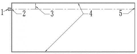
1- nozzle inlet, 2- nozzle outlet, 3- distance between fluid core and wall surface, 4- wall surface in the computational domain, 5- outlet surface in the computational domain
Figure 3. Single-nozzle water jet model
It can be seen from Figure 3 that the single-nozzle water jet model included the following structures: 1, nozzle inlet; 2, nozzle outlet; 3, distance between fluid core and wall surface; 4, wall surface in the computational domain; 5, outlet surface in the computational domain. The fluid medium water entered the water tank from nozzle inlet 1 and was ejected from nozzle outlet 2 and hit wall surfaces 4 and outlet surface 5 from all directions. There’re certain distances between the fluid core of the water jet and the upper and lower wall surfaces 4 of the water tank. Since the relative distances of upper and lower wall surfaces 4 were fixed, the distance between fluid core and wall surface 3 (distance 3) was taken as the research object. The water tank wall surface 4 was the space boundary condition that restricted the fluid medium water ejected from the nozzle outlet; the distance 3 was an important parameter studied in this paper, it was defined as a variable set in the simulation calculation. In order to obtain different distances 3, multiple models of single-nozzle water jet had been constructed for simulation and calculation, so as to study the influence of distance 3 on the wall effect of water tank. According to the characteristics of fluid flow, the model size, the computation amount and time, and other factors were considered comprehensively, when distance 3 was a relatively small value between 0-3mm, the value interval was relatively small as well, it took 0mm, 1mm, 2mm, and 3mm, respectively; at the same time, two larger representative distances of 5mm and 10mm were also chosen for the simulation calculation.
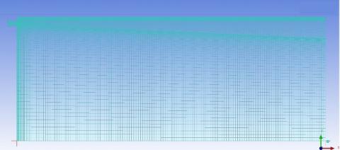
The single-nozzle water jet model was divided into meshes; and the single-nozzle water jet mesh model is shown in Figure 4.
As can be seen from Figure 4, the model was composed of regular grids, there were 4238 units and 8484 nodes in the model. In order to study the wall effect of automotive water tank more accurately, the grids near the wall surface of the water tank and the nozzle were denser.
FLUENT software is a professional fluid field analysis software with plenty physical models, advanced numerical methods, powerful pre- and post-processing functions, and secondary development functions; it has the advantages of wide application range, high efficiency and time saving, good stability and high precision, therefore it has been widely used in the fields of aerospace, automotive design, oil and gas, and turbine design, etc. This paper applied FLUENT software to simulation calculation, and made following assumptions about the simulation model in the calculation:
(1) The calculation used the pressure-based steady-state calculation method, and the fluid was Newtonian fluid;
(2) The calculation models were the VOF two-phase flow model and the RNG k-epsilon model. In order to better simulate the wall effect, the Scalable Wall Function was adopted in the calculation;
(3) The fluid boundary conditions were: the inlet pressure was 1 MPa; the outlet pressure was the same as the ambient pressure, both were 0 MPa; the fluid media were water medium and air medium included in the FLUENT software; to make the simulation calculation more accurate, the cavitation effect of water was considered in the model.
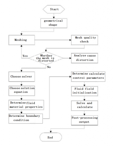
The specific simulation calculation flow in FLUENT is shown in Figure 5 below.
Figure 4. Single-nozzle water jet mesh model
Figure 5. Simulation calculation flow in FLUENT
4.1 Influence of wall effect on water jet direction and wall pressure
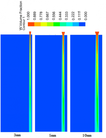
The distributions of total fluid field of medium water under the conditions of different distances between the fluid core and the upper wall surface obtained through simulation calculation are shown in Figure 6.
It can be seen from Figure 6 that, among the distribution maps, the maximum volume fraction of water was 100% and the minimum volume fraction of water was 0%; under the conditions of different distances, the distribution positions of the maximum volume fraction were different as well. As the distance between the fluid core and the upper wall surface increased, at a same water jet distance, the volume fraction of the water fluid became smaller; the water stream gradually moved away from the upper wall surface at the distal end of the nozzle, and the direction of the water stream changed more easily. The reason for the above phenomenon was that the space between the water stream and the wall surface of the water tank was relatively limited. When the water flowed on the edge of the space at a higher speed, the air near the water inside the water tank was taken away by the water stream due to the entrainment effect, resulting in pressure decrease in this space; as the distance of the water jet increased, the velocity of the water jet gradually decreased, and the direction of the water stream changed more easily as well.
The distribution of pressure on the upper wall surface of the water tank under different differences between fluid core and upper wall surface obtained through simulation calculation is shown in Figure 7.
Figure 6. Distribution of the total fluid field of medium water at different distances between fluid core and upper wall surface
Figure 7. Distribution of pressure on the upper wall surface under the condition of different distances between fluid core and upper wall surface
It can be seen from Figure 7 that, at a same distance between fluid core and upper wall surface, with the increase of the water jet distance, the pressure on the upper wall surface showed a trend of increasing first, decreasing later, then remaining unchanged, and decreasing in the end; when the distance between fluid core and upper wall surface was 1 mm, the pressure on the upper wall surface reached a maximum value of 3640Pa at a water jet distance of 0.025mm; when the distance between fluid core and upper wall surface was 2mm, the pressure on the upper wall surface reached a maximum value of 3690Pa at the water jet distance of 0.025mm, too. At a same water jet distance, for different distances between fluid core and upper wall surface, the pressures on the upper wall surface of the water tank were different as well. The reason for the above phenomenon was that at the position where the distance of the water jet was 0.025mm, the water from the water jet was ejected onto the upper wall surface in a large amount, resulting in higher pressure on the upper wall surface at the position, moreover, due to the influence of the upper wall surface, the direction of the water jet changed greatly.
4.2 Influence of wall effect on jet velocity
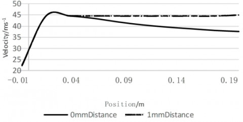
The distribution of water jet velocity under the condition of different distances between fluid core and upper wall surface obtained via simulation calculation is shown in Figure 8.
Figure 8. Distribution of water jet velocity under the condition of different distances between fluid core and upper wall surface
It can be seen from Figure 8 that, at a same distance between fluid core and upper wall surface, with the increase of water jet distance, the water jet velocity showed a trend of increasing first and decreasing later; when the distance between fluid core and upper wall surface was 0mm and 1mm, the water jet velocity reached a maximum value of 46.5m/s at a water jet distance of 0.01 mm. When distance between fluid core and upper wall surface was 0mm, the water jet velocity decreased, this was because the water jet stream had been attached to the wall surface of the water tank, and the viscous effect between the wall surface and the water had caused the water jet velocity to decrease.
4.3 Wall effect between water jet streams
Based on the wall effect of the single-nozzle water jet in automotive water tank studied above, in order to better study the wall effect between the water jet streams, a double-nozzle water jet model was constructed as shown in Figure 9.
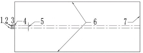
As can be seen from Figure 9, the double-nozzle water jet model included the following structures: inlet of nozzle-1, inlet of nozzle-2, outlet of nozzle-1, outlet of nozzle-2, distance between the two nozzles, the wall surface in the computational domain, and the outlet surface in the computational domain. The fluid medium water entered the water tank from inlets of nozzles 1 and 2, and was ejected from outlets of nozzles 1 and 2, and hit the wall surface and outlet surface from all directions. In the model of Figure 9, the boundary conditions and nozzle structure parameters of the two nozzles were the same. The model was divided into meshes in the same way as the single-nozzle water jet model, and the obtained mesh model for two-nozzle water jet is shown as Figure 10.
1, inlet of nozzle-1; 2, inlet of nozzle-2; 3, outlet of nozzle-1; 4, outlet of nozzle-2; 5, distance between the two nozzles; 6, wall surface in the computational domain; 7, outlet surface in the computational domain
Figure 9. Double-nozzle water jet model
Figure 10. Double-nozzle water jet mesh model
It can be seen from Figure 10 that the model was composed of regular grids, there were 5387 units and 11026 nodes in the model. In order to study the wall effect of automotive water tank more accurately, the grids of the wall surface near the nozzles were denser.
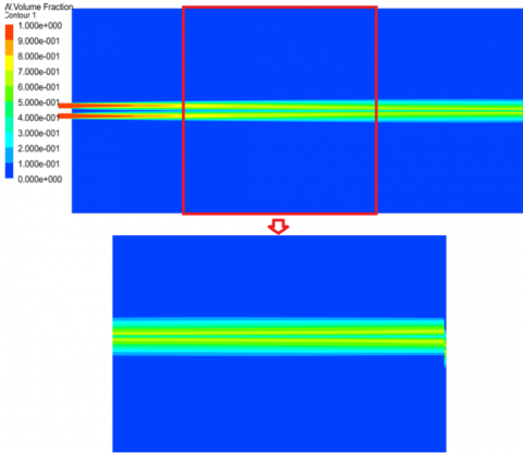
The same calculation method and flow of the single-nozzle model were adopted, after simulation calculation, the obtained distribution of the total fluid field of water medium when the distance between nozzles was 4mm is shown in Figure 11.
It can be seen from Figure 11 that when the distance between the two nozzles was 4mm, at the distal end of the nozzles, the two water jet streams converged, indicating that wall effect also existed between the flowing water streams, but the convergence position was far away from the nozzles.
Figure 11. Distribution of total fluid field of water medium when the distance between the two nozzles was 4mm
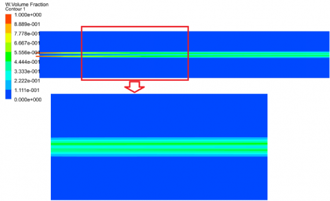
The distribution of total fluid field of water medium when the distance between the two nozzles was 2 mm is shown as Figure 12.
Figure 12. Distribution of total fluid field of water medium when the distance between the two nozzles was 2mm
It can be seen from Figure 12 that when the distance between the two nozzles was 2 mm, the two water jet streams converged at the distal end of the nozzles, too. By comparing Figures 11 and 12 we can know that, when the distance between the nozzles decreased from 4mm to 2mm, the convergence position of the water jet streams got closer to the position of the nozzles. It can be seen that the two water jet streams would converge when they were close to each other, and the smaller the distance between the nozzles, the earlier the convergence would occur, which was consistent with the wall effect of the water tank.
This paper constructed an uncertainty model for the fluid field in the automotive water tank, conducted secondary development in the FLUENT software according to the theoretical model, and then constructed models for the single-nozzle and double-nozzle automotive water tanks to simulate the characteristics of the water jet in the fluid field of automotive water tank. Through the study of the water jet and wall effect in the automotive water tank, it’s found that when water approached the wall surface of the water tank, the wall effect would occur; after the water contacted the wall surface, due to the damping generated by the wall surface, the velocity of the water was decreased. Therefore, the position of the nozzle should be optimized during the water jet-related design and its engineering application, so as to reduce or use the wall effect on the water flow.
In the simulation of two-nozzle water jet, it’s found that when the two nozzles were close to each other, the two water streams would converge, and its law was consistent with the wall effect of the water tank. This phenomenon would reduce the jet surface of the water jet, but it would increase the water jet distance and velocity. Therefore, when designing automotive water tank with multiple nozzles, the mutual interference between water streams should be taken into consideration.
The above research provided an important reference for automotive water tank optimization, water tank parameter optimization, water tank service life extension, and the application of fluid field theory in various industries.
This work is supported by “Funding Project for High-End Training of Professional Leaders in Higher Vocational Colleges, Jiangsu Province (Grant numbers: 2019GRGDYX118)” And “QingLan Project in Jiangsu Province”.
[1] Asfandiyar, Cai, B.W., Zhuang, H.L., Tang, H.C., Li, J.F. (2020). Polycrystalline SnSe–Sn1–vS solid solutions: Vacancy engineering and nanostructuring leading to high thermoelectric performance. Nano Energy, 69: 104393. https://doi.org/10.1016/j.nanoen.2019.104393
[2] O'Connor, K.P., Smitherman, A.D., Milton, C.K., Palejwala, A.H., Lu, V.M., Johnston, S.E., Homburg, H., Zhao, D., Martin, M.D. (2020). Surgical Treatment of Tethered Cord Syndrome in Adults: A Systematic Review and Meta-Analysis. World Neurosurgery. https://doi.org/10.1016/j.wneu.2020.01.131
[3] Cao, S.L., Buchholz, K., Tan, P.M., Aboelkassem, Y., Stowe, J.C., Saucerman, J.J., Omens, J., McCulloch, A.D. (2020). Analysis of differential gene expression in response to anisotropic stretch using a systems model of cardiac myocyte mechanotransduction. Biophysical Journal, 118(3): 459a-460a.
[4] Li, J., Liu, R.H., Yuan, P., Pei, Y.L., Cao, R.J., Wang, G. (2020). Numerical simulation and application of noise for high-power wind turbines with double blades based on large eddy simulation model. Renewable Energy, 146: 1682-1690. https://doi.org/10.1016/j.renene.2019.07.164
[5] Rochling Automotive SE & Co. KG; "Multi-Part Injection-Molded Multi-Chamber Plastic Tank Having an Oblique Joining Surface" in Patent Application Approval Process (USPTO 20190184815). Energy Weekly News, 2019.
[6] Iiyama, K., Yoshiyuki, A., Fujita, K., Ichimura, T., Morikawa, H., Hori, M. (2019). A point-estimate based method for soil amplification estimation using high resolution model under uncertainty of stratum boundary geometry. Soil Dynamics and Earthquake Engineering, 121: 480-490. https://doi.org/10.1016/j.soildyn.2018.11.028
[7] Chandramouli, P., Heitz, D., Laizet, S., Mémin, E. (2018). Coarse large-eddy simulations in a transitional wake flow with flow models under location uncertainty. Computers and Fluids, 168: 170-189. https://doi.org/10.1016/j.compfluid.2018.04.001
[8] Winiarski, M.J., Kurnatowska, M. (2018). Electronic structure of Ce1-xMxO2, where M=Rh, Pd, by MBJLDA calculations. Solid State Sciences, https://doi.org/10.1016/j.solidstatesciences.2018.09.016
[9] Fan, M.Y., Hu, J.W., Cao, R.S., Ruan, W.Q., Wei, X.H. (2018). A review on experimental design for pollutants removal in water treatment with the aid of artificial intelligence. Chemosphere, 200: 330-343. https://doi.org/10.1016/j.chemosphere.2018.02.111
[10] Córcoles-Tendero, J.I., Belmonte, J.F., Molina, A.E., Almendros-Ibáñez, J.A. (2018). Numerical simulation of the heat transfer process in a corrugated tube. International Journal of Thermal Sciences, 126: 125-136. https://doi.org/10.1016/j.ijthermalsci.2017.12.028
[11] Verkade, J.S., Brown, J.D., Davids, F., Reggiani, P., Weets, A.H. (2017). Estimating predictive hydrological uncertainty by dressing deterministic and ensemble forecasts; a comparison, with application to Meuse and Rhine. Journal of Hydrology, 555: 257-277. https://doi.org/10.1016/j.jhydrol.2017.10.024
[12] Kumaran, S.T., Ko, T.J., Uthayakumar, M., Islam, M.M. (2017). Prediction of surface roughness in abrasive water jet machining of CFRP composites using regression analysis. Journal of Alloys and Compounds, 724: 1037-1045. https://doi.org/10.1016/j.jallcom.2017.07.108
[13] Harless, A., Franz, E., Breuer, M. (2017). Heat transfer and friction characteristics of fully developed gas flow in cross-corrugated tubes. International Journal of Heat and Mass Transfer, 107: 1076-1084. https://doi.org/10.1016/j.ijheatmasstransfer.2016.10.129
[14] Sydeman, W.J., Thompson, S.A., Anker-Nilssen, T., Arimitsu, M., Bennison, A., Bertrand, S., Boersch-Supan, P. (2017). Best practices for assessing forage fish fisheries-seabird resource competition. Fisheries Research, 194: 209-221. https://doi.org/10.1016/j.fishres.2017.05.018
[15] Henry, A., Sattizahn, J.R., Norman, G.J., Beilock, S.L., Maestripieri, D. (2017). Performance during competition and competition outcome in relation to testosterone and cortisol among women. Hormones and Behavior, 92: 82-92. https://doi.org/10.1016/j.yhbeh.2017.03.010
[16] Xu, K., Zeng, Y.B., Li, P., Zhu, D. (2015). Study of surface roughness in wire electrochemical micro machining. Journal of Materials Processing Tech, 222: 103-109. https://doi.org/10.1016/j.jmatprotec.2015.03.007