Aftab Ahmed | Fareed Hussain Mangi* | Muhammad Kashif | Faheem Akhtar Chachar | Zia Ullah
© 2020 IIETA. This article is published by IIETA and is licensed under the CC BY 4.0 license (http://creativecommons.org/licenses/by/4.0/).
OPEN ACCESS
Proton Exchange Membrane Fuel Cell is considered one of the best alternatives to conventional sources of energy especially for automobile industry but faces heat and mass transfer challenges limiting its market penetration. This study investigates the effect of different parameters on the performance of a fuel cell with serpentine type single channel geometry using 3-D numerical simulations of the fuel cell model in the academic version of ANSYS Fluent 18.1. The fuel cell domain was discretized using structured hexagonal mesh with 150 K elements after a mesh independence study of the model. Numerous simulations were run for a temperature range of 298 K to 353 K, pressure between 1 to 3 bar and humidity ratio between 20%-80% to isolate the effect of transport phenomena on the performance of fuel cell. The effects of non-uniform temperature and pressure distributions due to varying mass flow rate were also studied. It was concluded that for the proposed design a mass flow rate of 0.8 mg/s at a pressure of 2.5 bar results in high current density, better water and heat removal, and reasonable pressure drop across the flow channels.
proton exchange membrane fuel cell, computation fluid dynamics, non-isothermal flow
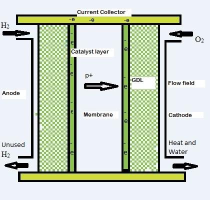
Proton exchange membrane fuel cells (PEMFCs) are widely used in military equipment, stationary applications and buses due to their compactness, high power density, and absence of noise and pollutant emissions. It is a device which converts chemical energy of hydrogen into electrical power through electrochemical reactions in an enclosed cell. A fuel cell consists of a membrane separating fuel (hydrogen) from the oxidizer (Oxygen), and allows the transfer of ions only. A catalyst layer, gas diffusion layer, and bipolar plate on both sides of membrane are used to accelerate the breakdown of fuel and oxidizer molecules into anions and cations. The gas enters through flow fields carved inside bipolar plates and reaches catalyst layer after passing through gas diffusion layer. The hydrogen breaks into protons releasing electron which takes an external conduction path and generate an electric current. The hydrogen enters from anode side and after the reaction electrons, protons and oxygen meet at cathode side [1]. Figure 1 shows the schematic representation of a typical fuel cell while the simplified reaction mechanism is given in Eqns. (1)- (3).
However, a typical PEM fuel cell suffers from some of the drawbacks which need to be resolved for the commercialization of this clean technology. Heat and water management are the critical issues directly linked to the serviceable life and performance of fuel cell. The recombination reaction taking place at the cathode is an exothermic reaction which raises the temperature of the cell and without an effective heat management system might lead to overheating of the cell.
The temperature variation between cell and operating environment may cause serious consequences including melting [2]. The rise in temperature also causes dehydration of membrane and loss in current density because temperature increases resistance to the flow of electrons through bipolar plates.
Figure 1. Schematic representation of various parts of a PEMFC and direction of flow of fuel and oxidizer and the resulting current produced. GDL stands for gas diffusion layer
On the other hand, the excessive water produced at cathode side mainly causes flooding of flow fields and reduces reaction site area requiring a strategy to remove this water without dehydrating the membrane [3].
Anode: $H_{2}(g) \rightarrow 2 H^{+}(a q)+2 e^{-}$ (1)
Cathode: $\frac{1}{2} O_{2}(g)+2 H^{+}(a q)+2 e^{-} \rightarrow 2 H_{2} O(l)$ (2)
Overall Reaction: $H_{2}(g)+\frac{1}{2} O_{2}(g) \rightarrow H_{2} O(l)+heat+electrcity$ (3)
The parallel flow channel geometry of fuel cell has simple and durable design, which makes it a strong candidate for automobile applications. The multiphase flow phenomenon within flow field may lead to more complicated operating conditions in order to mitigate thermal, water management and mass transport issues [4]. Different techniques can be used to overcome flooding and dehydration problem. Dehydration of membrane can be reduced by humidifying reactant gases and flooding can be reduced by using higher flow velocity on cathode side. The higher inlet velocity will increase convection heat transfer that will also solve the heating problem in some cases [5]. A lot of research effort is dedicated to understand the effect of operating parameters on fuel cell performance in order to achieve the maximum efficiency and optimal power. In this regard numerical simulations offer a cheap and efficient alternative to experimentation for the optimization of operating conditions such as flow velocity, inlet conditions, temperature gradient and humidity for optimized fuel cell performance. Higher mass flow rate causes significant loss in gain due to increase in pressure drop across the fuel cell and require an efficient channel design that shows relatively smaller increase in pressure drop with increasing mass flow rate of reactants [6]. Numerical simulations of PEM fuel cells are performed in this study to reveal the effects of operating parameters on fuel cell performance.
This study outlines a methodology to numerically simulate the operation of a PEM fuel cell using commercially available software. This study also describes a strategy to identify optimum operating conditions and the impact of reactant flow rates on the operation of the cell. The main objective is to identify design parameters and operating conditions that results in higher current densities form the fuel cell while ensuring lower temperatures, humidification of membrane and avoiding flooding in the cathode side flow channels. The paper also discusses the impact of temperature and pressure on fuel cell parameters at constant flow rate. The novelty of the work lies in the simultaneous estimation of the effect of flow rate, operating pressure and humidity ratio on the performance of a PEM fuel cell employing a computationally light simulation technique. The results of the study are analyzed to identify the effect of serpentine channel design, flow rate, humidity ratio on the performance of PEM fuel cell and recommend optimum values of these parameters. In addition, this study used 3D flow fields and geometry to observe whether oxygen starvation problem improves or not by varying mass flow-rate of anode and cathode flow-rates.
The design of PEM fuel cell used in current study and the model setup is explained in the methodology section, the results of the parametric study and the selection of optimum operating parameters in included in the results and discussion section. At the end main conclusions reached by analyzing the results of this numerical study have been given along with future recommendations.
A three-dimensional model of a PEM fuel cell consists of a number of equations that are used to simulate fluid flow, gas diffusion, electrochemical process and transport of water and other gases.
The simplified model used here for the simulation assumes that the flow is steady and laminar with all the gases and vapors following ideal gas equation. All the water generated as the result of the reaction of hydrogen with oxygen is in gaseous form. The model equations have been developed and used by many researchers and are easily available in the fuel cell module manual of ANSYS fluent 18.1 [7] and also in literature [8-14]. The governing equations and PEM fuel cell sub-models are given in the following sections.
2.1 Continuity equation
The conservation of mass or continuity equation for a three-dimensional compressible flow is given by Eq. (4).
$\frac{\partial(\rho u)}{\partial x}+\frac{\partial(\rho v)}{\partial y}+\frac{\partial(\rho w)}{\partial z}=-\frac{\partial \rho}{\partial t}$ (4)
where, u, v and w are velocities in the x, y and z direction respectively, $\rho$ is density of reactant gases. Taking into account the porosity of electrodes and membrane this equation transforms to Eq. (5).
$\frac{\partial(\rho \epsilon u)}{\partial x}+\frac{\partial(\rho \epsilon v)}{\partial y}+\frac{\partial(\rho \epsilon w)}{\partial z}=S_{m}$ (5)
$S_{m}$ is the mass sink term and is zero except in the catalyst layer zone and are calculated for hydrogen, oxygen and water using Eqns. (6)-(8).
$S_{H_{2}}\left(k g s^{-1} m^{-3}\right)=\frac{M_{H_{2}}}{2 F} R_{a n}$ (6)
$S_{O_{2}}\left(k g s^{-1} m^{-3}\right)=\frac{M_{O_{2}}}{4 F} R_{c a t}$ (7)
$S_{H_{2 O}}\left(k g s^{-1} m^{-3}\right)=\frac{M_{H_{2} O}}{2 F} R_{c a t}$ (8)
Here, $F$ is the Faraday constant and $\mathrm{M}$ is the molecular weight of the species in $\mathrm{kg} / \mathrm{mol} . R_{a n}$ and $R_{c a t}$ is the exchange current density at the anode and cathode respectively.
2.2 Momentum equation
For porous electrodes, the general form of the momentum equation is given by Eq. (9).
$\nabla \cdot(\epsilon \rho \vec{v} \vec{v})=-\epsilon \nabla p+\nabla \epsilon \tau+S_{m o m}$ (9)
In x-direction, this equation transforms into Eq. (10).
$\begin{aligned} u \frac{\partial(\rho u)}{\partial x} &+v \frac{\partial(\rho u)}{\partial y}+w \frac{\partial(\rho u)}{\partial z} \\ &=-\frac{\partial p}{\partial x}+\frac{\partial}{\partial x}\left(\mu \frac{\partial u}{\partial x}\right)+\frac{\partial}{\partial y}\left(\mu \frac{\partial u}{\partial y}\right) \\ &+\frac{\partial}{\partial z}\left(\mu \frac{\partial u}{\partial z}\right)+S_{\operatorname{mom} x} \end{aligned}$ (10)
Here, $\vec{v}, p, \tau$ and $S_{m o m}$ are velocity vector, pressure, shear stress tensor, viscosity and momentum sink term respectively. Momentum term is zero in flow channels and for the porous zones of the model is given by Eq. (11).
$S_{\operatorname{mom}, x}=-\frac{\mu u}{\beta_{x}}$ (11)
where, $\beta$ is the permeability of the electrodes and is same in all having a value of $10^{-12} \mathrm{m}-12 .$ The momentum equations for y and z directions can be easily formulated by replacing appropriate terms in Eqns. (10) and (11).
2.3 Mass transfer equations
The continuity equation for a certain species i is given by Eq. (12).
$\nabla \cdot\left(\rho \vec{v} y_{i}\right)=-\nabla \cdot \vec{\jmath}_{i}+S_{i}$ (12)
The diffusion mass flux j can be calculated using Fick’s law as given by Eq. (13).
$\overrightarrow{J_{i}}=-\sum_{j=1}^{N-1} \rho D_{i j} \nabla \overrightarrow{y_{i}}$ (13)
Within the porous electrodes mass transfer equation for any species can be written as given by Eq. (14).
$\nabla \cdot\left(\rho \epsilon \vec{v} y_{i}\right)=\nabla \cdot\left(\rho \epsilon D_{i j}^{e f f} \nabla y_{i}\right)+S_{i}$ (14)
where, $y_{i}$ is the mass fraction of species i (H2, O2, and H2O.) diffusivity can be estimated using modified Brueggemann equation (Eq. (15)).
$D_{i j}^{e f f}=D_{i j} \times \epsilon^{1.5}$ (15)
The mass transfer equations for all species has the following general form as given by Eq. (16).
$\begin{aligned} u \frac{\partial\left(\rho y_{i}\right)}{\partial x} &+v \frac{\partial\left(\rho y_{i}\right)}{\partial y}+w \frac{\partial\left(\rho y_{i}\right)}{\partial z} \\ &=\frac{\partial\left(j_{x, i}\right)}{\partial x}+\frac{\partial\left(\rho j_{y, i}\right)}{\partial y}+\frac{\partial\left(j_{z, i}\right)}{\partial z} \\ &+S_{i} \end{aligned}$ (16)
2.4 Mass transfer equations
The rate of change of energy can be modeled using Eq. (17)
$\nabla \cdot(\vec{v}(\rho E+P))=\nabla \cdot\left(k_{e f f} \nabla T-\sum_{j} h_{j} \vec{\jmath}_{j}+\right.$
$\left.\left(\tau_{e f f} \cdot \vec{v}\right)\right)+S_{h}$ (17)
Here $E, h, \boldsymbol{\tau}_{e f f}$ are the total energy, enthalpy and effective shear tensor respectively. $k_{e f}$ is the effective thermal conductivity and can be calculated using Eq. (18) from the thermal conductivity of the fluid, $\left(k_{f}\right)$ and solid, $\left(k_{s}\right)$.phases.
$k_{e f f}=\epsilon k_{f}+(1-\epsilon) k_{f}$ (18)
Sh is the sink term and can be calculated using Eq. (19).
$S_{h}=h_{p h a s e}+h_{r e a c t i o n}+R_{o h m} I^{2}$ (19)
where, hphase is neglected as there is no phase change modeled and hreaction is zero in bipolar plate as there is no reaction. Hence Eq. (20) can be used to estimate the temperature change.
$\nabla \cdot(k \nabla T)=-R_{o h m} I^{2}$ (20)
Here k is the thermal conductivity of the bipolar plate.
2.5 Charge conservation equations
Electrochemical reactions occur in the fuel cell that generate current and the driving force behind these reactions is the surface activation over-potential, $\phi$ The conservation of electron and ions is modeled in the solid parts and in membrane using Eqns. (21) and (22).
$\nabla \cdot\left(\sigma_{s o l} \nabla \phi_{s o l}\right)+R_{s o l}=0$ (21)
$\nabla \cdot\left(\sigma_{m e m} \nabla \phi_{m e m}\right)+R_{m e m}=0$ (22)
$\sigma$ is Electrical conductivity of membrane or solid phase of the fuel cell model and Rsol and Rmem are the volume sink terms or current density (A/m3) and are given by set of Eqns. (23)-(26).
Anode side: $R_{s o l}=-R_{a n}(<0)$ (23)
and
$R_{m e m}=R_{a n}(>0)$ (24)
Cathode side: $R_{s a l}=R_{c a t}(>0)$ (25)
and
$R_{m e m}=-R_{c a t}(<0)$ (26)
These terms can be calculated using Butler-Volmer equations (Eqns. (27) and (28)).
$R_{a n}=R_{a n}^{e f f}\left(\frac{C_{H_{2}}}{C_{H_{2}}^{r e f}}\right)^{\gamma a n}\left(e^{\left(\frac{\alpha_{a n} F}{R T}\right) \eta_{a n}}-e^{\left(\frac{\alpha_{c a t} F}{R T}\right) \eta_{c a t}}\right)$ (27)
$R_{c a t}=R_{c a t}^{e f f}\left(\frac{C_{O_{2}}}{C_{O_{2}}^{r e f}}\right)^{\gamma c a t}\left(e^{\left(\frac{\alpha_{c a t} F}{R T}\right) \eta_{c a t}}-e^{\left(\frac{\alpha_{a n} F}{R T}\right) \eta_{a n}}\right)$ (28)
Average current density is calculated from Eq. (29).
$i_{a v e}=\frac{1}{A} \int_{V_{a n}} R_{a n} d V=\frac{1}{A} \int_{V_{c a t}} R_{c a t} d V$ (29)
The water content of the membrane can be estimate using Eq. (30).
$\lambda=\left\{\begin{array}{l}0.043+17.81 a+39.85 a^{2}+36 a^{3}, 0 \leq a \leq 1 \\ 14+1.4(a-1)\end{array}, 0 \leq a \leq 1\right.$ (30)
2.6 Water transport through membrane
The water generated as a result of the reaction of hydrogen with the oxygen at the cathode of a PEM fuel cell diffuse towards the anode due to electro-osmosis and back diffusion. To reduce the computation time and load, single phase was assumed and all the water formed was considered to be in gaseous form.
This section provides the mechanical design of the fuel cell and the steps and methods for setting up a numerical model using appropriate boundary conditions. The details of different parameters and PEM fuel cell sub-models used by ANSYS Fluent 18.1 are also provided at the end of this section.
The mechanical design of a PEM fuel cell is quite simple however, the fluid flow, heat transfer and electrochemical reactions occurring inside cell make simulation a challenging task. The numerical simulation of a PEM fuel cell includes the design of fuel cell geometry specifying the flow areas, meshing of the geometry and setting boundary conditions and other simulation parameters [8, 9]. The fuel cell used in this study has flow channels of constant cross-section of 0.8 mm × 0.8 mm and an isometric view of the fuel cell mechanical design is shown in Figure 2. The main dimensions of the fuel cell are resumed in Table 1.
Figure 2. Schematic representation of the design of a single channel PEMFC
The parallel flow channel geometry was designed using a commercial 3-D modelling software and was imported and meshed into ANSYS 18.1. The fuel cell geometry is suitable for structured mesh. The final meshed fuel cell domain had about 150k elements. A mesh independent study was also performed and revealed that increasing elements number beyond 150k elements had negligible effect on simulation results. The built-in model for PEMFC module of ANSYS Fluent was used for this simulation word. The PEMFC model contains sub models of Joule heating, Reaction heating, butler-volmer rate and membrane water transport to simulate heat transfer, fluid phenomenon and chemical reactions. The advantage of using this particular model is that it provides wide range of sub models which help in all diverse phenomenon occurring within fuel cell compared to other limited use models. The selection of appropriate materials for membrane and other parts is a vital part of the simulation. The fluid flow and heat transfer are solved using CFD with help of conservation of mass, momentum and energy equations. The SIMPLE algorithm was chosen for calculation of solution.
Table 1. Dimensions of different fuel cell parts
|
|
Length (mm) |
Width (mm) |
Thickness (mm) |
|
Current collector |
40 |
2 |
2 |
|
Membrane |
40 |
2 |
0.0241 |
|
Catalyst layer |
40 |
2 |
0.010 |
|
Channels |
40 |
0.8 |
0.8 |
|
GDL |
40 |
2 |
0.041 |
Table 2. The operating Parameters of the fuel cell including geometric dimensions
|
|
Parameter |
Value |
|
Bipolar plate |
Density |
2.0 g/cm3 |
|
Electrical conductivity |
100 s.cm-1 |
|
|
Thermal conductivity |
10 w m-1 k-1 |
|
|
thickness |
2 mm |
|
|
Gas diffusion layer |
Density |
0.35-0.45 g/cm3 |
|
Porosity |
0.5 |
|
|
thickness |
0.041 mm |
|
|
Catalyst layer |
thickness |
0.010 mm |
|
Membrane |
Specific gravity |
1.97 |
|
Ionic conductivity |
0.2 s/cm |
The model parameters and boundary conditions specified in Table 2 were used for the simulation and remain constant throughout the study [10]. While, the boundary conditions applied to the model for simulation of PEM fuel cell are given in Table 3.
In addition, the flows of on the anode and cathode sides were incompressible and laminar and water condensation was not included. All the gases were treated as ideal gas and ideal gas law was used for the calculations of thermodynamic properties [11]. The novelty of the work lies in the parametric analysis performed here to reveal the optimized operating pressure, mass flow rate and humidity ratio of anode and cathode side flows.
The built-in models of incompressible laminar flow of ANSYS fluent employs equations of conservation of mass, momentum and energy to solve the fluid flow and heat problem. Also, the built-in single phase, steady state PEMFC model equations such as Joule heating, Reaction heating, Butler volmer and membrane water transport are solved to simulate the working of a PEM fuel cell. There were nine parts in the geometry and all were considered as fluid except the bipolar plates. The under-relaxation factors were adjusted to stabilize the solution. The water content and water saturation were set 0.95 and pressure and momentum as 0.3. The solution was chosen to run in double precision mode. Different planes were created to get the values of different local parameters of the fuel cell at different locations after the convergence of the solution.
Table 3. Boundary conditions specification in the fluent for the simulation of PEM fuel cell
|
BC types |
Location |
Parameters |
Values |
Units |
|
Anode |
Anode-inlet |
Mass flow rate (H2 and H2O) |
6e-07 |
Kg/s |
|
Temperature |
353 |
K |
||
|
Mass fraction H2 |
0.8 |
|
||
|
Water saturation |
0 |
|
||
|
Cathode |
Cathode-inlet |
Mass flow rate (O2 and H2O) |
5e-06 |
Kg/s |
|
Temperature |
353 |
K |
||
|
Mass fraction O2 |
0.6 |
|
||
|
Water saturation |
0 |
|
||
|
Pressure-outlets |
Anode-cathode-outlets |
Operating pressure |
1-3 |
bar |
|
Gauge Pressure |
0 |
bar |
||
|
Temperature |
353 |
K |
||
|
Terminal-a |
The top surface of the current collector |
Temperature |
353 |
K |
|
Electric potential |
0 |
V |
||
|
Terminal-c |
The top surface of the current collector |
Temperature |
353 |
K |
|
Electric potential |
0.65 |
V |
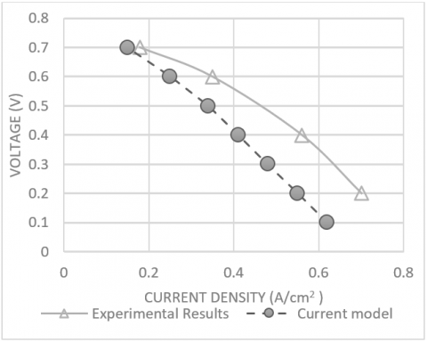
The results of the numerical simulations were interpreted and then analyzed by plotting various output parameters of the fuel cell against the operating pressure, mass flow rates and temperatures. A detail analysis is provided here based on the numerical study of the varying operating conditions on the performance, current output, hydrogen consumption etc. of a PEM fuel cell. The reliability of the numerical simulations is ensured by comparing the results with experimental results obtained from the literature as shown in Figure 3.
Figure 3. The comparison of polarization curve of the simulated fuel cell with an experimentally measured data
The issues of a PEM fuel cell such as heat and water management, losses due to pressure and temperature gradient have been studied using numerical simulations. The results of PEMFC simulations can help solve challenges and require accurate prediction of the effect of operating conditions on fuel cell operation. In a PEM fuel cell, all three fundamental phenomena such as heat transfer, fluid flow and electrochemical reaction are directly or indirectly dependent on mass flow rates. An increase in mass flow rate at cathode side may have positive impact on heat transfer while on the other hand a reduced mass flow rate may result in less unused fuel at the fuel channel outlet. It may also affect the water content inside the cathode flow channel.
The polarization curve is the basic performance indicator of a PEM fuel cell being simulated numerically in this study. Figure 3 shows the polarization curve based on simulation values showing cell voltage as a function of current density and agrees well experimental results [15]. This validation clearly shows the capability of the PEM fuel cell model used for current simulations. The single value of current density was achieved at each iteration performed and shows a difference of less than 10% from the experimentally determined values.
Figure 4. The impact of mass flow rate on current density with increasing operating pressure
The effect of increasing mass flow rate and pressure on current density is shown in Figure 4. The results of the simulation show that the combine effect of increasing mass flow rate and pressure has a direct impact on fuel cell performance. The current shows a linear increase with pressure from 1 atm to 3 atm. The optimum values of mass flow rate and pressure were found to be 0.0008 g/s and 2.5 atm respectively. Any further increase in mass flow rate results in increased velocity and the heat transfer at bipolar plate also increases. This results in fewer hot areas on the anode side as compared to the cathode side that could be due to lower mass flow rate on the cathode side. On the other hand, it decreases efficiency and lowers fuel consumption rate that ultimately impacts the overall performance and also increased pressure drop across the channel. The inflection points on the curves of current density and change in mass fraction of hydrogen at the outlet, thus corresponds to optimum parameters for a fuel cell as analyzed in detailed here.
Another reason may be the recombination reaction occurring at the cathode side releasing more heat as the cathode current density increases. Any further increase in mass flow rate or operating pressure beyond the optimum values reported above show an increase in the current density to a small extent but it also resulted in more water content at cathode flow field that might cause flooding problem on the cathode side channel.
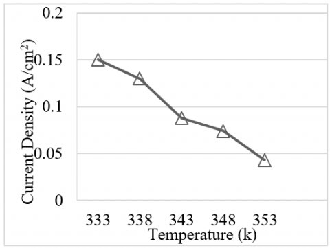
Figure 5 shows the effect of temperature on current density while keeping the mass flow rates constant. As the temperature of the fuel cell increases the current density decreases due to increased resistance to the flow of electrons. The increasing temperature may increase reaction kinetics at catalyst layer but it affects negatively when electrons travel through bipolar plate. The suitable operating temperature for PEM fuel cell when flow rate and operating pressure were kept constant was observed to be 343 k. The current density drops suddenly if temperature is further increased because benefit of higher kinetics is lost as resistances due to hot spots.
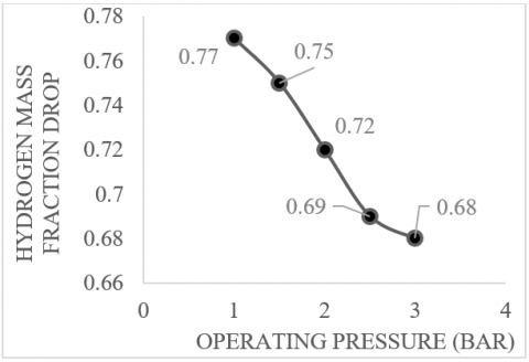
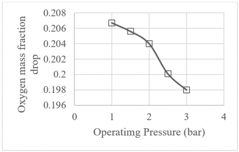
The mass fraction of hydrogen and oxygen at the fuel cell outlet is a good indicator of the performance of a PEM fuel cell. The mass fraction of hydrogen at the outlet is shown in Figure 6 at different operating pressures. The result of this numerical study shows that the mass fraction of hydrogen at the outlet decreases at a high rate with increasing pressure until 2.5 atm and then the curve starts to level out if the pressure is increased further. This shows increased consumption of hydrogen in the fuel cell that enhances the performance of the fuel cell. With the increasing pressure there is higher convection of gas through gas diffusion layer resulting in an increase of reaction rate at the catalyst layer. The lower change in mass fraction was observed at 1 atm compared to 2 atm inside anode flow channel as more fuel was consumed at higher operating pressure and decrease in mass fraction was higher. The same trend was observed inside cathode flow channel where at 1 atm less mass fraction change was observed compared to 2 atm as shown in Figure 6. The decrease in mass fraction of reactants improved from 13% to 23% as the operating pressure was changed from 1 to 2 atm. However, pressure drop inside flow channels also increased when operating pressure was raised as shown in Figure 7.
Figure 8 depicts the pressure drop inside flow field hence overall reduction during different operating conditions can be estimated from above distribution. Furthermore, it is evident from the image that during initial turns of serpentine pressure drop is less compared to end of geometry. The reason is that friction becomes dominant hence pressure drop is maximum at end of channels.
Figure 5. The impact of temperature on current density when flow rate is constant
Figure 6. The impact of operating pressure on mass fraction drop
Figure 7. The drop in oxygen mass fraction
Figure 8. The pressure distribution inside multiple serpentine flow channels. The values of pressure are relative to atmospheric pressure and not absolute pressure
Numerical investigation of a PEM fuel with parallel channels of constant cross section and opposite flow has been performed in ANSYS fluent 18.1. The effect of the variation in mass flow rate of humidified hydrogen and oxygen on the performance of fuel cell has been revealed. The performance of the fuel cell was improved significantly when flow rate was increased along with operating pressure. The higher current density values were achieved at 6×10⁻⁷ kg/s and 2.5 bar pressure without the problem of excessive heat and water both on anode and cathode side. The conditions of fuel cell during these operating conditions were also observed to be stable and fewer hot spots were seen in the results of the simulations. The key finding of the current study was that smaller flow channels dimensions cause less polarization concentration at higher current densities.
The water content inside flow channel also reduced. However, pressure across flow channel increases with increase in operating pressure hence that may add parasite load on the fuel cell. The variation in mass flow rate also affects the temperature within flow channel and at bipolar plate. The small difference in temperature was observed from heat source to current collector plates. This study provides some useful insight into the effect of different parameters on the operation and performance of a PEM fuel that could help improve the design of a fuel cell.
The simulations were performed assuming steady state, laminar flow conditions to reduce computational time and cost. More detailed and specific studies on the effect of various geometries of the flow channels can help in exploring further avenues for the performance enhancement of future PEM fuel cell using numerical simulations. Also, the effect of turbulence and mixing on the performance should be studied by running unsteady fluid flow simulations. Higher order discretization models and coupling methods can be used to further increase the accuracy of the numerical simulations. However, this will result in increased computational cost and time and will require a cluster of high-end computers to perform a parametric study to analyze the effect of operating parameters on proton exchange membrane fuel cell.
The authors would like to thank Sukkur IBA University for providing licensed software and support for this project.
|
A |
Area $\left(m^{2}\right)$ |
|
C |
Concentration, (mol. $m^{-3}$ ) |
|
F |
Faraday Constant, $\left(C . m o l^{-1}\right)$ |
|
k |
Thermal conductivity, $\left(W \cdot m^{-1} \cdot K^{-1}\right)$ |
|
M |
Molecular weight, $\left(g . m o l^{-1}\right)$ |
|
R |
Exchange current density $\left(g . m o l^{-1}\right)$ |
|
S |
Sink source |
|
u |
Velocity in x direction, $\left(m . s^{-1}\right)$ |
|
V |
Velocity in y direction, $\left(m . s^{-1}\right)$ |
|
w |
Velocity in z direction, $\left(m . s^{-1}\right)$ |
|
Greek symbols |
|
|
$a$ |
Charge transport coefficient |
|
$\beta$ |
Electrode permeability, (m2) |
|
$\phi$ |
Activation overpotential (V) |
|
$\sigma$ |
Electrical conductivity, (S.m-1) |
|
$\lambda$ |
Water content of membrane |
|
$\mu$ |
Dynamic viscosity (kg s m−2) |
|
$\rho$ |
Density (kg.m-3) |
|
$\epsilon$ |
Porosity |
|
Subscripts |
|
|
an |
Anode |
|
cat |
Cathode |
|
mem |
Membrane |
|
sol |
Solution |
|
f |
Fluid |
|
s |
Solid |
|
(l) |
Liquid phase |
|
(g) |
Gaseous phase |
|
eff |
Effective |
[1] Barbir, F. (2006). PEM fuel cells. Fuel Cell Technology, 27-51. https://doi.org/10.1007/1-84628-207-1_2
[2] Djilali, N., Lu, D. (2002). Influence of heat transfer on gas and water transport in fuel cells. International Journal of Thermal Sciences, 41(1): 29-40. https://doi.org/10.1016/S1290-0729(01)01301-1
[3] Mosdale, R., Srinivasan, S. (1995). Analysis of performance and of water and thermal management in proton exchange membrane fuel cells. Electrochimica Acta, 40(4): 413-421. https://doi.org/10.1016/0013-4686(94)00289-D
[4] Prater, K.B. (1992). Solid polymer fuel cell developments at Ballard. Journal of Power Sources, 37(1-2): 181-188. https://doi.org/10.1016/0378-7753(92)80076-N
[5] Owejan, J.P., Gagliardo, J.J., Sergi, J.M., Kandlikar, S.G., Trabold, T.A. (2009). Water management studies in PEM fuel cells, Part I: Fuel cell design and in situ water distributions. International Journal of Hydrogen Energy, 34(8): 3436-3444. https://doi.org/10.1016/j.ijhydene.2008.12.100
[6] Yadava, M.K., Sahub, B.R., Gupta, B., Bhattb, S. (2013). Effect of mass flow rate and temperature on the performance of PEM fuel cell: an experimental study. International Journal of Current Engineering and Technology (IJCET), 3.
[7] Wang, Y., Chen, K.S., Mishler, J., Cho, S.C., Adroher, X.C. (2011). A review of polymer electrolyte membrane fuel cells: Technology, applications, and needs on fundamental research. Applied Energy, 88(4): 981-1007. https://doi.org/10.1016/j.apenergy.2010.09.030
[8] Arvay, A. (2011). Proton exchange membrane fuel cell modeling and simulation using Ansys Fluent. Arizona State University, America.
[9] Arvay, A., French, J., Wang, J.C., Peng, X.H., Kannan, A.M. (2015). Modelling and simulation of biologically inspired flow field designs for proton exchange membrane fuel cells. The Open Electrochemistry Journal, 6(1). https://doi.org/10.2174/1876505X01506010001
[10] Oh, K., Chippar, P., Ju, H. (2014). Numerical study of thermal stresses in high-temperature proton exchange membrane fuel cell (HT-PEMFC). International Journal of Hydrogen Energy, 39(6): 2785-2794. https://doi.org/10.1016/j.ijhydene.2013.01.201
[11] Penga, Ž., Tolj, I., Barbir, F. (2016). Computational fluid dynamics study of PEM fuel cell performance for isothermal and non-uniform temperature boundary conditions. International Journal of Hydrogen Energy, 41(39): 17585-17594. https://doi.org/10.1016/j.ijhydene.2016.07.092
[12] Arvay, A., Ahmed, A., Peng, X.H., Kannan, A.M. (2012). Convergence criteria establishment for 3D simulation of proton exchange membrane fuel cell. International Journal of Hydrogen Energy, 37(3): 2482-2489. https://doi.org/10.1016/j.ijhydene.2011.11.005
[13] Wang, L., Husar, A., Zhou, T., Liu, H. (2003). A parametric study of PEM fuel cell performances. International Journal of Hydrogen Energy, 28(11): 1263-1272. https://doi.org/10.1016/S0360-3199(02)00284-7
[14] Wilberforce, T., Khatib, F.N., Ijaodola, O.S., Ogungbemi, E., El-Hassan, Z., Durrant, A., Olabi, A.G. (2019). Numerical modelling and CFD simulation of a polymer electrolyte membrane (PEM) fuel cell flow channel using an open pore cellular foam material. Science of The Total Environment, 678: 728-740. https://doi.org/10.1016/j.scitotenv.2019.03.430
[15] Badduri, S.R., Srinivasulu, G.N., Rao, S.S. (2019). Computational fluid dynamic analysis on PEM fuel cell performance using bio channel. In Materials Science Forum, 969: 524-529. https://doi.org/10.4028/www.scientific.net/MSF.969.524