Nuttawee Pengpom | Somsak Vongpradubchai | Phadungsak Rattanadecho*
© 2019 IIETA. This article is published by IIETA and is licensed under the CC BY 4.0 license (http://creativecommons.org/licenses/by/4.0/).
OPEN ACCESS
Air pollution adversely influences health of human, especially the indoor air pollution being poor ventilation. This article studied the carbon dioxide concentration dispersion and convective heat transfer in the two-dimensional factory model affected by different convective heat transfers and pollutant concentration levels. The continuity equation, momentum equations, heat transfer equation, and species concentration equation for an unsteady state are numerically solved based on the finite element method. The simulation results are found that the inlet air velocity is the main factor affecting the pollutant concentration dispersions. The effect of the air temperature on pollutant dispersion is greater at higher temperature difference between the inlet air temperature and the initial temperature. The average pollutant concentration ratios in the factory are similar. Although, the average pollutant concentrations in the factory increases with the pollutant concentration levels. The obtained results can apply in the prediction of pollutant concentration dispersion and ventilation system management.
pollutant concentration dispersion, convective heat transfer, inconstant diffusion coefficient, factory model, indoor air pollution
Pollution has been a significant problem that affects our health, especially indoor air pollution. There are many kinds of pollution sources such as combustion process, cooking, smoking, and other sources [1]. Breathing the air contaminated with pollutants can make you ill such as irritation, headache, dizziness, and fatigue [2-4].
In the past, there were many researches to study the pollutant concentration dispersion both outdoor and indoor pollution. The outdoor pollution has been studied about the effects of pollutants concentration on urban and river. Vasile et al. [5, 6] studied the pollution in a river and decreasing the pollutant concentration by using a neutralizing agent in order to counteract the pollutant spreading effect in the river. The pollution in the river was numerically solved by a simulation program based on the finite element method. Gualtieri, Carlo [7] studied the pollution simulation based on Reynolds Average Navier-Stokes (RANS), and the simulated results were verified by comparing with the experimental results. The preliminary results simulating the transverse mixing of steady state in two-dimensional rectangular geometry were presented. Amorim et al. [8] studied the effects of trees on pollutant concentration in the urban models. The pollutant concentration dispersion was calculated based on the RANS and URban VEgetation (URVE). From this research, the different wind directions and urban models can affect the pollutant concentration dispersion.
The indoor air has been studied about the ventilation efficiency both with and without air pollution. The most researches have studied the ventilation efficiency without air pollution. Theses researches always studied the effects of temperature, moisture, pressure, air velocity, directions of flow and other variables on ventilation efficiency [9-12]. After that, analyzing the ventilation systems are considered together with the indoor air pollution. There are many variables can affect the indoor air pollution. Zheming et al. [13] studied the effects of outdoor air pollution on the indoor air pollution based on Large Eddy Simulation (LES) with unsteady turbulent flow. Increasing the distance between building and road can decrease particle concentration in the indoor building. However, the particle concentration may depend on the other variables such as particle size, wind direction, inlet area size and location of inlet. The effects of inlet and outlet have been studied. Qi-Hong Deng et al. [14] studied the effects of the strength of heat source (Gr), the strength of contaminant source (Br), the strength of external ventilation (Re), and the position of the outlet. This research numerically investigated the fluid, heat and pollutant transport structures in a two-dimensional and laminar flow model. The outlet located nearest the pollution source with high forced convection is the best case for removing the pollutant and heat out of the model. Shi-Jie Cao et al. [15] studied the influence of ventilation rates on the indoor air quality with buoyancy force effect based on RANS. An increase in the inlet ventilation rate can increase the impact on pollutant concentration. Shui Yu et al. [16] numerically studied eliminating benzene pollutant of four different natural ventilation strategies by using Airpak 3.0 simulation program in order to find the suitable ventilation strategies. The four different natural ventilation strategies are varied by the size of the windows of the residential building. The three-dimensional residential model was simulated by computational fluid dynamics (CFD) with steady state k-e turbulent model. The pollutant concentration decreases with the sum of the area sizes of inlets. Mao Ning et al. [17] studied the effects of the located heights of the supply air outlet on the ventilation. This article used the CFD simulation program with the SST turbulence model. The lower located heights of the supply air outlet are better for saving energy and removing the pollutant in a breathing zone. Although, the temperature of the whole room decreases with located height of the supply air outlet. Mohamad Kanaan and Khaled Chahine [30] studied the effects of different ventilation schemes in ventilating electrical rooms based on finite volume method. Their study shown that the decrease in height of the exhaust fans can improve the cooling effect. Wufeng Jin et al. [18] studied the ventilation of R32 concentration leaking from a floor type air conditioner. The R32 concentration is inversely proportional with the heights of outlet because the density of R32 is higher than the density of air. Therefore, the outlet should be located at the lower heights. Moreover, the high pollutant concentration on the same height plane always occurs in the corner of the room. The position and size of the inlet and outlet are significant for managing the pollutant concentration dispersion. However, changing the ventilation systems are difficult when the room or building was already built. Ruining Zhuang et al. [19] studied the effects of furniture layouts and the positions of inlet and outlet on the indoor air quality. There were three different furniture layouts and four different ventilation systems. The formaldehyde concentration dispersion is simulated by ANSYS 13.0 with the turbulent model as RNG k-e in the three-dimensional model. Changing the furniture layout can affect the air flow field, temperature distribution, and formaldehyde concentration dispersion. The pollution source located nearest the outlet is the best case. Yu Shui et al. [20] studied the effects of the different location of the purifier, different purification efficiency and different opening time on formaldehyde concentration dispersion. The purifier located nearest the pollution source is appropriate to reduce the pollutant concentration in the whole room. Keramatollah Akbari et al. [21, 22] studied the effects of temperature, relative humidity, pressure difference, and ventilation rate on the indoor radon. The obtained results are simulated by FLUENT CFD package with steady state laminar and turbulent flow in the three-dimensional model. The ventilation rate and temperature are inversely proportional with the radon concentration. An increase in the relative humidity can decrease the radon concentration. However, the radon concentration increases when the relative humidity is higher than 70 percentages. The radon concentration dispersion in the whole room increases with the pressure difference. However, Keramatollah Akbari et al. [23] studied the effects of ventilation on radon concentration. The pressure jump in exhaust fan considered between 2-20 pascal is inversely proportional with the radon concentration. Van Schijndel [24] considered the different simulation methods as finite element method (FEM), building energy simulation (BES) and state-space (SS) in order to investigate the efficiency of the methods. These simulation methods numerically solve heat transfer, moisture, and pollution. However, the finite element method did not still consider the effects of moisture and pollutant concentration dispersion.
This article studied the combined pollutant concentration dispersion and convective heat transfer in the two-dimensional factory model. Moreover, the diffusion coefficient of the pollutant in this study depends on the temperature. This study is different from some articles studied only the effects of the ventilation on pollutant concentration. The CO2, contaminated in air, concentration has three different levels emitted from both furnaces. In addition, the factory is affected by the different air velocities and the different inlet air temperatures of the factory. The governing equations with the unsteady state were numerically calculated by the simulation program based on the finite element method (FEM). The model was verified with the results of the previous researches. This article aimed to study the relation of variables, the variation of variables with time and analyzation to find the main variable affecting the velocity, temperature and pollutant concentration for the ventilation system management in the factory model.
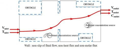
This article studied the combined pollutant concentration dispersion and convective heat transfer in the two-dimensional factory model (Figure 1). The CO2, contaminated in air, is emitted from high fixed temperature furnaces. Moreover, the factory is affected by the convective heat transfer at the inlet of the factory.
2.1 Governing equations
This article studied the combined pollutant concentration dispersion and convective heat transfer in the two-dimensional factory model with an unsteady state.
The continuity equation and momentum equations define the characteristic of flow. In addition, the heat transfer equation is also studied. This model is affected by the convective heat transfer at the inlet and the high fixed temperature at the surfaces of both furnaces. Analysis of the convective heat transfer is assumed that:
(1) The characteristics of fluid flow are laminar and compressible.
(2) The body force from gravity and buoyancy force is not included.
(3) The factory is not affected by the radiation from the outdoor environment.
(4) There is no phase change of the fluids.
The continuity equation
$\frac{\partial \rho}{\partial t}+\frac{\partial \rho u}{\partial x}+\frac{\partial \rho v}{\partial y}=0$ (1)
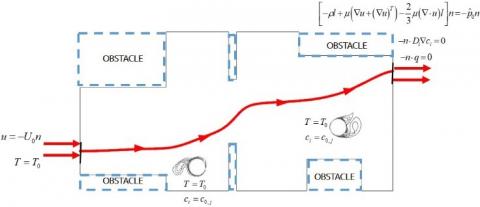
(a) Boundary conditions
(b) Boundary condition equations
Figure 1. Geometry and boundary conditions of the model
The momentum equations
$\frac{\partial \rho u}{\partial t}+u \frac{\partial \rho u}{\partial x}+v \frac{\partial \rho u}{\partial y}=-\frac{\partial p}{\partial x}$ (2)
$\frac{\partial \rho v}{\partial t}+u \frac{\partial \rho v}{\partial x}+v \frac{\partial \rho v}{\partial y}=-\frac{\partial p}{\partial y}$ (3)
The heat transfer equation
$\rho c_{p}\left(\frac{\partial T}{\partial t}+u \frac{\partial T}{\partial x}+v \frac{\partial T}{\partial y}\right)=\frac{\partial}{\partial x}\left(k \frac{\partial T}{\partial x}\right)+\frac{\partial}{\partial y}\left(k \frac{\partial T}{\partial y}\right)$ (4)
where r is the density of air (kg.m-3), u and v are the velocity of fluid (m.s-1), cp is the specific heat capacity (J.kg-1. K-1), p is the pressure (Pa), T is the temperature (K) and k is the thermal conductivity (W.m-1.K-1).
The three different inlet air temperatures quote from the approximated temperatures of each season in Thailand. The initial temperature inside the factory is 27 °C.
(1) The inlet air temperature of 21.2 °C is the lowest temperature in the winter and lower than the initial temperature.
(2) The inlet air temperature of 28.2 °C is the average temperature in the rainy season and approximates to the initial temperature.
(3) The inlet air temperature of 36.2 °C is the highest temperature in the summer and higher than the initial temperature.
The inlet air velocity quotes from Modeling indoor air pollution written by Darrell W Pepper and David Carrington (2009) [25]. Moreover, this study adds two different values to analyze the effects of different inlet air velocities.
(1) The inlet air velocity equals 1.0 m.s-1 quoting from Modeling indoor air pollution written by Darrell W Pepper and David Carrington (2009) [25].
(2) The inlet air velocity equals 0.7 m.s-1 (70% of 1 m.s-1).
(3) The inlet air velocity equals 1.3 m.s-1 (130% of 1 m.s-1).
The species concentration equation derives from Fick’s first law of diffusion in the conditions that the diffusion coefficient is constant and no flow, Eq. (5).
$N=-\left(D \frac{\partial C}{\partial x}+D \frac{\partial C}{\partial y}\right)$ (5)
The Fick’s second law can derive from the continuity of mass, Eq. (6).
$\frac{\partial C}{\partial t}=\frac{\partial}{\partial x}\left(D \frac{\partial C}{\partial x}\right)+\frac{\partial}{\partial y}\left(D \frac{\partial C}{\partial y}\right)$ (6)
The assumptions of pollutant concentration dispersion are:
(1) The pollutant is the carbon dioxide contaminating the air.
(2) The air and carbon dioxide do not react with each other.
(3) The carbon dioxide consisted of air is neglected.
The species concentration equation for unsteady time and constant diffusion coefficient can be written as Eq. (7).
$\frac{\partial C}{\partial t}+u \frac{\partial C}{\partial x}+v \frac{\partial C}{\partial y}=\frac{\partial}{\partial x}\left(D_{x x} \frac{\partial C}{\partial x}\right)+\frac{\partial}{\partial y}\left(D_{y y} \frac{\partial C}{\partial y}\right)+S$ (7)
where N is the molar flux (mol.m-2.s-1), D is the diffusion coefficient (m2.s-1), C is the pollutant concentration (mol.m-3) and S is the pollutant concentration emitted from the pollution source (mol.m-3.s-1).
In this article, there are three different concentration levels (C0) of carbon dioxide emitted from both furnaces as shown below [26]:
(1) Level 1: 0.1 mol.m-3 of pollutant concentration sources can cause a headache, sleepiness and stagnant.
(2) Level 2: 0.5 mol.m-3 of pollutant concentration sources is the highest concentration limit that human can endure. Moreover, it can lead to oxygen deprivation.
(3) Level 3: 1.0 mol.m-3 of pollutant concentration level contribute to oxygen deprivation immediately.
The diffusion coefficients of air-carbon dioxide depending on temperature are shown in Table 1. [27].
Table 1. Binary diffusion coefficient (m2.s-1)
|
T (K) |
O2 |
CO2 |
H2 |
NO |
|
200 |
0.95 |
0.74 |
3.75 |
0.88 |
|
300 |
1.88 |
1.57 |
7.77 |
1.80 |
|
400 |
5.25 |
2.63 |
12.5 |
3.03 |
|
500 |
4.75 |
3.85 |
17.1 |
4.43 |
|
600 |
6.46 |
5.37 |
24.4 |
6.03 |
|
700 |
8.38 |
6.84 |
31.7 |
7.82 |
|
800 |
10.5 |
8.57 |
39.3 |
9.78 |
|
900 |
12.6 |
10.5 |
47.7 |
11.8 |
|
1000 |
15.2 |
12.4 |
56.9 |
14.1 |
|
1200 |
20.6 |
16.9 |
77.7 |
19.2 |
|
1400 |
26.6 |
21.7 |
99.0 |
24.5 |
|
1600 |
33.2 |
27.5 |
125 |
30.4 |
|
1800 |
40.3 |
32.8 |
152 |
37.0 |
|
2000 |
48.0 |
39.4 |
180 |
44.8 |
Note: The diffusion coefficients are refered from CENGEL, Yunus A., 2015; Table 14-1, p. 840
2.2 Numerical procedures
The numerical study of the combined pollutant concentration dispersion and convective heat transfer in the two-dimensional factory model is solved by a simulation program based on the finite element method (FEM). COMSOL MultiphysicsTM is the simulation program to solve these equations in this study [28].
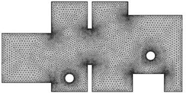
An investigation of mesh independence at a measured point (20, 10) is found that the number of elements is 12,683 elements. The characteristic of elements is the triangular element. The maximum element size is 0.56 m, and the minimum element size is 0.008 m (Figure 2).
Figure 2. Finite element mesh based on computational model
The validation of the pollutant concentration dispersion is verified by comparing with the maximum of pollutant concentration at several points in the research of Gualtieri [7]. Their research studied based on finite element method with the RANS equations. An independence mesh of the k-ϵ turbulent model of 52,734 elements and of the laminar flow of 19,046 elements. The characteristic of flow was the k-ϵ turbulent model. The validation result is similar although, the maximum values of pollutant concentration away from the pollutant source are different. The errors are 10.04 % for the k-ϵ turbulent model and 5.56 % for the laminar flow model. This result is shown in Figure 3.
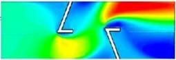
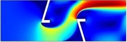
The validation of the convective heat transfer is verified by comparing with research of Menni and et al. [29]. Their research studied the effect of the baffle L-shape with Reynolds numbers between 12,000 to 30,000 based on finite volume method (FVM). The validation is comparison with the result as Reynold number of 12,000. An independence mesh of this model of 12,200 elements. Comparing the patterns of convective heat transfer shows that the patterns are similar (Figure 4).
Therefore, these validations can be an acceptable results. The different result may be caused by the incomplete simulation data of the previous articles.
Figure 3. Comparison of the maximum pollutant concentration
(a) Simulation result of Menni and et al.
(b) Validation result
Figure 4. Comparison of the velocity fields
The obtained results from studying the combined pollutant concentration dispersion and convective heat transfer in the two-dimensional factory model are demonstrated in Section 4.1-4.4.
4.1 Effects of heat transfer on pollutant concentration dispersion
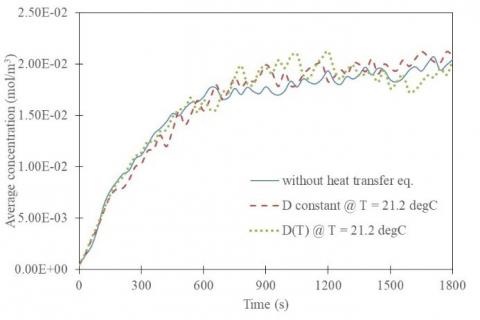
The effects of heat transfer on pollutant concentration dispersion are shown in Figure 5. In the first period, the average pollutant concentrations in factory analyzed together with the heat transfer equation are lower than the average pollutant concentration in factory analyzed without the heat transfer equation. This is because their average diffusion coefficients are lower than the diffusion coefficient of the case analyzed without the heat transfer equation. After that, the temperature in the whole factory increases, and the diffusion coefficient also increases. Therefore, in the last period, the average pollutant concentrations in factory analyzed together with the heat transfer equation are higher than the average pollutant concentration in factory analyzed without the heat transfer equation. However, the average pollutant concentrations in the factory are still similar.
In this article studied the combined pollutant concentration and the convective heat transfer in the two-dimensional factory model. Moreover, the diffusion coefficient depends on the temperature (Table 1). The obtained results are demonstrated in Section 4.2-4.4.
Figure 5. Comparison of different analysis
4.2 Temperature distributions
The inlet air temperature and the high fixed temperature at the surface of both furnaces highly affect the temperature distributions in the factory. In the first period, the high temperature occurs around both furnaces due to the effect of the high fixed temperature at the surface of both furnaces. However, it is decreased by the effect of inlet air temperature. After that, the temperature in the whole factory increases due to the effects of inlet air temperature and high fixed temperature at the surface of both furnaces (Figure 6). This is because these temperatures are higher than the initial temperature.
The effects of the inlet air temperatures on temperature distributions are shown in Figure 7. An increase in the inlet air temperature raises the temperature in the whole factory, especially the temperature around the first furnace. However, each temperature distribution is similar. Additionally, the average temperature in the factory is higher at higher inlet air temperature (Figure 8). The average temperatures in the factory are higher than the initial temperature. Although, in the first period, some inlet air temperature being lower than the initial temperature decrease the average temperature in the factory to be lower than the initial temperature.
Figure 6. Temperature distributions varying with time
Figure 7. Temperature distributions affected by inlet air temperatures of 21.2, 28.2 and 36.2 °C
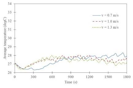
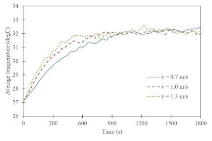
The effects of the inlet air velocity on temperature distributions are shown in Figure 9. An increase in the inlet air velocity decreases the temperature around both furnaces when the inlet air temperatures are lower than the initial temperature. Contrarily, the increase in the inlet air velocity increases more temperature in the other area when the inlet air temperatures are higher than the initial temperature. In the first period, the average temperature in the factory is higher at higher inlet air velocity. However, in the last period, most of the average temperatures in the factory are similar, except for the inlet air temperatures being lower than the initial temperature. Its average temperature in the factory is lower at higher inlet air velocity (Figure 8).
The effects of the pollutant concentration levels on temperature distributions are shown in Figure 10. The concentration levels can slightly affect the temperature distributions and the average temperatures in the factory (Figure 11).
Therefore, the inlet air temperature is the main factor affecting the temperature distributions and the average temperatures in the factory. The temperature distributions are similar. The high temperature always occurs around both furnaces due to the effect of the high fixed temperature at the surface of both furnaces.
(a) Inlet air temperature of 21.2 °C
(b) Inlet air temperature of 28.2 °C
Figure 8. Average temperatures in the factory
Figure 9. Temperature distributions affected by inlet air velocities of 0.7, 1.0 and 1.3 m.s-1
Figure 10. Temperature distributions affected by pollutant concentration levels of 0.1, 0.5 and 1.0 mol.m-3
Figure 11. Average temperatures affected by pollutant concentration levels
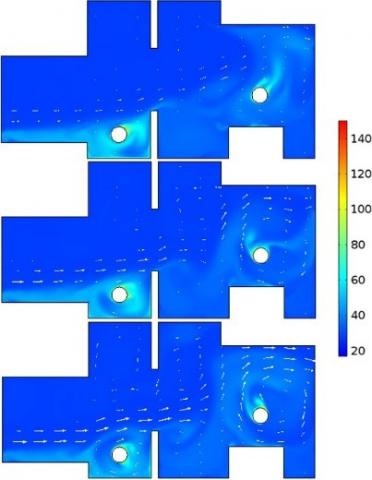
4.3 Velocity fields
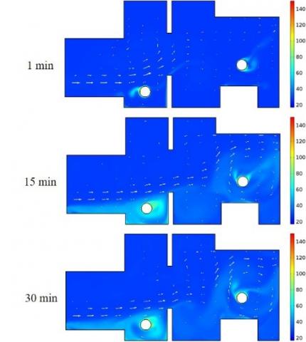
The primary flow flows from the inlet to the outlet of the factory and slows down after it flows through the first furnace. Meanwhile, the secondary flows occur throughout the factory. The velocity at the outlet of the factory is high due to the effects of high pressure within the factory. The patterns of velocity fields in the last period are more turbulent than the patterns of velocity fields in the first period (Figure 12).
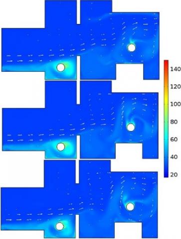
The effects of the inlet air temperature on velocity fields are shown in Figure 12. The inlet air temperatures can slightly affect the velocity fields. The velocity fields are similar. Although, an increase in temperature difference between the initial temperature and the inlet air temperature causes more turbulent flow and longer flow distance of the primary flow. Additionally, the average velocities in the factory are similar (Figure 13 (b)).
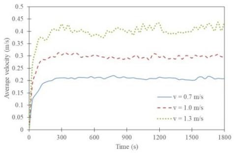
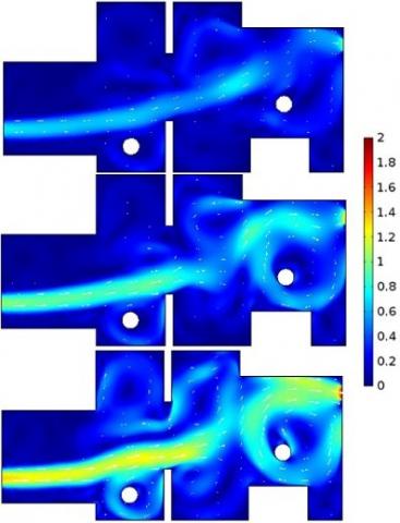
The effects of the inlet air velocity on velocity fields are shown in Figure 14. The increase in the inlet air velocity increases the air velocity, especially the velocity of primary flow. The flow distance of the primary flow is longer. However, the patterns of velocity fields are similar. Additionally, the average velocity in the factory is higher at higher inlet air velocity (Figure 13 (a)).
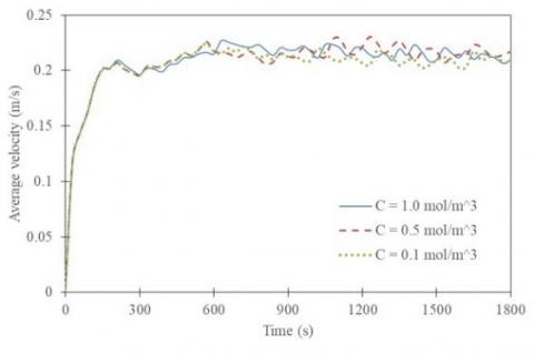
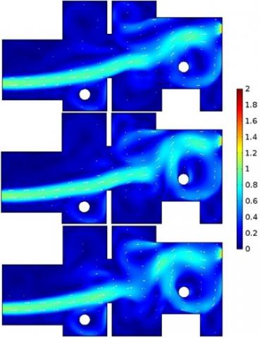
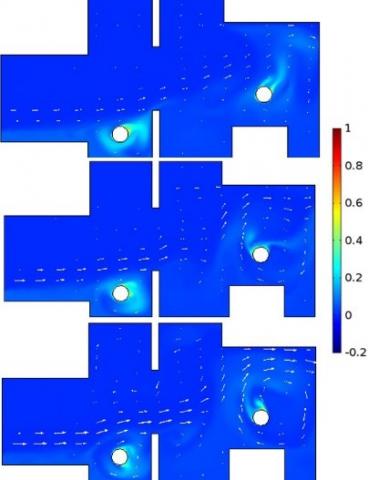
The effects of the pollutant concentration levels on velocity fields are shown in Figure 15. The increase in the pollutant concentration level can decrease more velocity of the primary flow after it flows through the first furnaces. However, the patterns of velocity fields are similar. Additionally, the average velocities in the factory are similar (Figure 13 (c)).
Therefore, the inlet air velocity is the main factor affecting the velocity field and the average velocity in the factory. The maximum velocity and the average velocity in the factory increase with the inlet air velocity.
Figure 12. Velocity fields varying with time
(a) Effects of the inlet air velocities
(b) Effects of the inlet air temperatures
(c) Effects of the pollutant concentration levels
Figure 13. Average velocities
Figure 14. Velocity fields affected by the inlet air velocities of 0.7, 1.0 and 1.3 m.s-1
Figure 15. Velocity fields affected by the pollutant concentration levels of 0.1, 0.5 and 1.0 mol.m-3
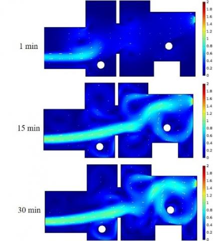
4.4 Pollutant concentration dispersions
The CO2 pollutant is constantly emitted from both furnaces. The pollutant concentration dispersions in the factory are affected by the convective heat transfer at the inlet. In the first period, the maximum pollutant concentration occurs around both furnaces, especially around the first furnace. This is because the pollutant concentration dispersion at the first furnace is affected by the convective heat transfer higher than at the second furnace, and the area under the primary flow of the first furnace is narrower than the area under the primary flow of the second furnace. In addition, the second furnace located near the outlet is easier for removing the pollutant, according to the research of Ruining Zhuang et al. [19]. In the last period, the CO2 pollutant spreads throughout the factory. However, the maximum pollutant concentration is still around both furnaces. The pollutant concentrations increase to a steady state during 15-20 minutes (Figure 16).
Figure 16. Pollutant concentration dispersions varying with time
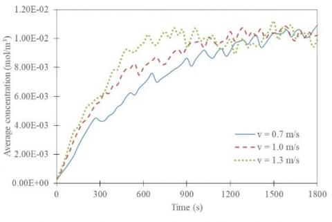
The effects of the inlet air velocity on pollutant concentration dispersions are shown in Figure 17. The pollutant concentration dispersions are similar. Although, they are slightly different at the first furnace. The pollution sources emit more pollutant at higher inlet air velocity. However, the increase in the inlet air velocity is also good for increasing the ventilation efficiency. Therefore, in the first period, the average pollutant concentration in the factory is higher at higher inlet air velocity. In the last period, it is lower at higher inlet air velocity (Figure 18).
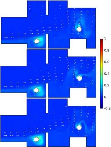
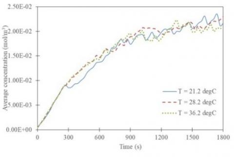
The effects of the inlet air temperature on pollutant concentration dispersions are shown in Figure 19. The increase in the inlet air temperature raises the pollutant concentration dispersion around the first furnace. This is because the diffusion coefficient property is proportional to the temperature. Additionally, the average pollutant concentrations in the factory affected by the inlet air temperature are shown in Figure 20. The average pollutant concentrations in the factory are similar.
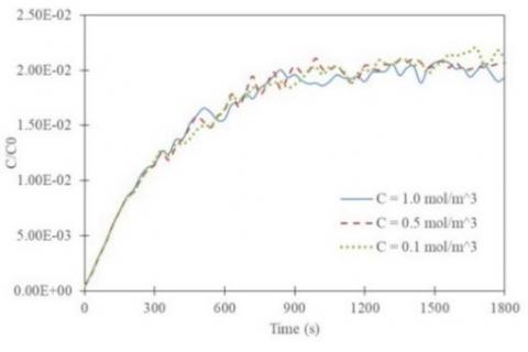
The effects of the concentration levels on pollutant concentration dispersions are shown in Figure 21. The pollutant concentration is higher at higher pollutant concentration level, especially around both furnaces. Additionally, the average pollutant concentration in the factory is higher at higher pollutant concentration level. However, the pollutant concentrations ratios of the average pollutant concentrations in the factory to the pollutant concentration levels are similar (Figure 22). Therefore, the pollutant concentration levels can slightly affect the pollutant concentration dispersions.
Figure 17. Pollutant concentration dispersions affected by inlet air velocities of 0.7, 1.0 and 1.3 m.s-1
Therefore, the inlet air velocity is the main factor affecting the pollutant concentration dispersion and the average pollutant concentration in the factory. Moreover, the pollutant concentration level can affect the average pollutant concentration in the factory. However, the pollutant concentration ratios of the average pollutant concentrations in the factory to the pollutant concentration levels are similar. The average pollutant concentration in the factory does not suddenly harm the health of human. However, the pollutant concentration around both furnaces is still dangerous.
(a) Inlet air temperature of 21.2 °C
(b) Inlet air temperature of 36.2
Figure 18. Average pollutant concentrations affected by inlet air velocities
Figure 19. Pollutant concentration dispersions affected by inlet air temperatures of 21.2, 28.2 and 36.2 °C
Figure 20. Average pollutant concentration affected by inlet air temperatures
Figure 21. Pollutant concentration dispersions affected by pollutant concentration levels of 0.1, 0.5 and 1.0 mol.m-3
(a) Pollutant concentration ratios affected by pollutant concentration levels
(b) Average pollutant concentrations affected by inlet air velocities
Figure 22. Comparison of the effects of pollutant concentration levels and inlet air velocities
This article studied the combined pollutant concentration dispersion and convective heat transfer in two-dimensional factory model, in order to study the effects of different convective heat transfers and pollutant concentration levels on the velocity fields, temperature distributions and pollutant concentration dispersions. The continuity equation, momentum equations, heat transfer equation, and species concentration equation for the unsteady time are numerically solved based on the finite element method.
The results show that the inlet air velocity is the main factor affecting the pollutant concentration dispersions. The average pollutant concentration in the factory is lower at higher inlet air velocity, especially in case of the high temperature difference between the inlet air temperature and the temperature in the whole factory. Moreover, the average pollutant concentration in the factory is higher at higher pollutant concentration level. However, the pollutant concentrations ratios are similar. The high pollutant concentration occurs around both furnaces, especially around the first furnace. The inlet air temperature is the main factor affecting the temperature distributions and the average temperatures in the factory. Also, the inlet air velocity is the main factor affecting the velocity fields and the average velocities in the factory. However, there are many variables that may affect these phenomena, such as wind direction, pressure difference, and the relative humidity.
Therefore, the results of this article can apply for predicting the phenomena of pollutant concentration dispersion and managing the ventilation systems.
The Thailand Research Fund (Contract No. RTA 5980009) and The Thailand Government Budget Grant provided financial support for this study.
|
A |
heat transfer area of surface, m2 |
|
cp |
specific heat, J. kg-1. K-1 |
|
C D |
pollutant concentration, mol.m-3 diffusion coefficient, m2.s-1 |
|
h |
convective heat transfer coefficient, W.m-2.K-1 |
|
k |
thermal conductivity, W.m-1. K-1 |
|
N |
molar flux, mol.m-2s-1 |
|
p |
pressure, Pa |
|
T |
temperature, °C |
|
u |
velocity of fluid in x-axis, m.s-1 |
|
v |
velocity of fluid in y-axis, m.s-1 |
|
Greek symbols |
|
|
$\rho$ |
density of fluid, kg.m-3 |
[1] Bernstein, J.A., Alexis, N., Barnes, C., Bernstein, I.L., Nel, A., Peden, D., Diaz-Sanchez, D., Tarlo, S.M., Williams, P.B. (2004). Health effects of air pollution. Journal of Allergy and Clinical Immunology, 114(5): 1116-1123. https://doi.org/10.1016/j.jaci.2004.08.030
[2] Persily, A.K. (1997). Evaluating building IAQ and ventilation with indoor carbon dioxide. Transactions-American Society of Heating Refrigerating and Air Conditioning Engineers, 103: 193-204.
[3] Seppänen, O., Fisk, W., Mendell, M. (1999). Association of ventilation rates and CO2 concentrations with health andother responses in commercial and institutional buildings. Indoor Air, 9(4): 226-252. https://doi.org/10.1111/j.1600-0668.1999.00003.x
[4] Jones, A.P. (1999). Indoor air quality and health. Atmospheric Environment, 33(28): 4535-4564. https://doi.org/10.1016/S1352-2310(99)00272-1
[5] Cristea, V.M., Bâgiu, E.D., Agachi, P.Ş. (2010). Simulation and control of pollutant propagation in Someş river using COMSOL multiphysics. Computer Aided Chemical Engineering, Elsevier, 28: 985-990. https://doi.org/10.1016/S1570-7946(10)28165-8
[6] Cristea, V.M. (2013). Counteracting the accidental pollutant propagation in a section of the River Someş by automatic control. Journal of Environmental Management, 128: 828-836. https://doi.org/10.1016/j.jenvman.2013.06.016
[7] Gualtieri, C. (2010). RANS-based simulation of transverse turbulent mixing in a 2D geometry. Environmental Fluid Mechanics, 10(1-2): 137-156. https://doi.org/10.1007/s10652-009-9119-6
[8] Amorim, J., Rodrigues, V., Tavares, R., Valente, J., Borrego, C. (2013). CFD modelling of the aerodynamic effect of trees on urban air pollution dispersion. Science of the Total Environment, 461: 541-551. https://doi.org/10.1016/j.scitotenv.2013.05.031
[9] Méndez, C., San José, J., Villafruela, J., Castro, F. (2008). Optimization of a hospital room by means of CFD for more efficient ventilation. Energy and Buildings, 40(5): 849-854. https://doi.org/10.1016/j.enbuild.2007.06.003
[10] Sudprasert, S., Chinsorranant, C., Rattanadecho, P. (2016). Numerical study of vertical solar chimneys with moist air in a hot and humid climate. International Journal of Heat and Mass Transfer, 102: 645-656. https://doi.org/10.1016/j.ijheatmasstransfer.2016.06.054
[11] Wang, Y., Meng, X., Yang, X., Liu, J. (2014). Influence of convection and radiation on the thermal environment in an industrial building with buoyancy-driven natural ventilation. Energy and Buildings, 75: 394-401. https://doi.org/10.1016/j.enbuild.2014.02.031
[12] Lu, W., Tam, C., Leung, A., Howarth, A. (2002). Numerical investigation of convection heat transfer in a heated room. Numerical Heat Transfer: Part A: Applications, 42(3): 233-251. https://doi.org/10.1080/10407780290059521
[13] Tong, Z., Chen, Y., Malkawi, A., Adamkiewicz, G., Spengler, J.D. (2016). Quantifying the impact of traffic-related air pollution on the indoor air quality of a naturally ventilated building. Environment International, 89: 138-146. https://doi.org/10.1016/j.envint.2016.01.016
[14] Deng, Q.H., Zhang, G. (2004). Indoor air environment: more structures to see? Building and Environment, 39 (12): 1417-1425. https://doi.org/10.1016/j.buildenv.2004.04.009
[15] Cao, S.J., Zhu, D.H., Yang, Y.B. (2016). Associated relationship between ventilation rates and indoor air quality. RSC Advances, 6(112): 111427-111435. https://doi.org/10.1039/C6RA22902F
[16] Yu, S., Zhang, G., Ma, Y., Yu, Z., Feng, G. (2017). Numerical simulation study on concentration distribution of indoor pollutions by different natural ventilation strategies in Shenyang. Procedia Engineering, 205: 1389-1396. https://doi.org/10.1016/j.proeng.2017.10.302
[17] Ning, M., Song, M.J., Chan, M.Y., Pan, D.M., Deng, S.M. (2016). Computational fluid dynamics (CFD) modelling of air flow field, mean age of air and CO2 distributions inside a bedroom with different heights of conditioned air supply outlet. Applied Energy, 164: 906-915. https://doi.org/10.1016/j.apenergy.2015.10.096
[18] Jin, W., Gao, P., Zheng, Y. (2017). Experimental study on ventilation effect on concentration distribution of R32 leaking from floor type air conditioner. Energy Procedia, 105: 4627-4634. https://doi.org/10.1016/j.egypro.2017.03.1003
[19] Zhuang, R., Li, X., Tu, J. (2014). CFD study of the effects of furniture layout on indoor air quality under typical office ventilation schemes. Building Simulation, 7(3): 263-275. https://doi.org/10.1007/s12273-013-0144-5
[20] Yu, S., Ma, Y.L., Zhang, G.J., Wang, W., Feng, G.H. (2017). Numerical simulation study on location optimization of indoor air purifiers in bedroom. Procedia Engineering, 205: 849-855. https://doi.org/10.1016/j.proeng.2017.10.024
[21] Akbari, K., Mahmoudi, J. (2012). Numerical simulation of radon transport and indoor air conditions effects. Int. J. Scientific and Engineering Research, 3(6): 1-9.
[22] Akbari, K., Mahmoudi, J. (2012). Effects of heat recovery ventilation systems on indoor radon. In: THE 25th International Conference on Efficiency, Cost, Optimization, Simulation and Environmental Impact of Energy System. June 26-29, 2012, PERUGIA, ITALY, 2012, pp 1-10.
[23] Akbari, K., Mahmoudi, J., Oman, R. (2012). Simulation of ventilation effects on indoor radon in a detached house. WSEAS Transactions on Fluid Mechanics, 7(4): 146-155.
[24] van Schijndel, A.J. (2017). Combining three main modeling methodologies for heat, air, moisture and pollution modeling. Energy Procedia, 132: 195-200. https://doi.org/10.1016/j.egypro.2017.09.754
[25] Pepper, D.W. (2009). Modeling indoor air pollution. Imperial College Press.
[26] Bonino, S. (2016). Carbon dioxide detection and indoor air quality control. Occupational Health & Safety (Waco, Tex.), 85(4): 46-48.
[27] Cengel, Y. (2015). Heat and mass transfer: Fundamentals and applications. Fifth edn. McGraw-Hill Higher Education.
[28] Comsol. (2014). COMSOL Multiphysics™ Version 4.4: User’s Guide and Reference Manual. Comsol Burlington, MA, USA,
[29] Menni, Y., Azzi, A., Zidani, C., Benyoucef, B. (2016). Numerical analysis of turbulent forced-convection flow in a channel with staggered L-shaped baffles. Journal of New Technology and Materials, 6(2):44-55.
[30] Kannan, M., Chahine, K. (2018). CFD study of ventilation for indoor multi-zone transformer substation. Internal Journal of Heat and Technology, 36(1): 88-94. https://doi.org/10.18280/ijht.360112