Alfan Sarifudin* | Danar Susilo Wijayanto | Indah Widiastuti
© 2019 IIETA. This article is published by IIETA and is licensed under the CC BY 4.0 license (http://creativecommons.org/licenses/by/4.0/).
OPEN ACCESS
The purpose of this study is to analyze the parameters of cold temperature and coefficient of performance refrigeration (COPref) of the vortex tube cooling machine and how much the contribution of each parameter to the performance. This analysis also aims to predict the optimal value of cold temperature and COPref of the vortex tube as well as to predict the condition of how the optimal value is obtained. To find out whether the analysis is suitable for optimizing the performance, then the confirmation data verification is done to know the error level. The parameters considered in the experiment were the tube type consisting of natural cooling and forced cooling, the pressures are 0.5bar, 1.0bar, and 1.5bar, and fractions are 30 %, 40 %, 50 %, 60 %, and 70 %. The results of the experimental test optimized using the Taguchi method where data is reduced by selecting the three optimal fractions in each response. Obtained that tube type, pressure, and fraction are factors that influence performancewith the level of error for predicting the optimal value at cold temperatures is <5 %. This study provides an analysis of the contribution of improved design of vortex tube performance parameters that are efficient experimental and reliable statistics.
could temperature, coefficient of performance refrigeration (COP), cooling machine, natural cooling, forced cooling, parameter design, efficient experimental and reliable statistics
Current cooling machine needs cannot be separated from daily life. One of the cooling devices used in the industrial world is vortex tube. This tool can only be used with compressible air that is sprayed, so this tool is very environmentally friendly because it does not produce dangerous freon emissions. Vortex tube in a works system has no moving parts therefore it does not require maintenance costs for wear components due to friction, which makes it more economical in maintenance [1].
Many research efforts to improve the performance of this tool have been carried out. It was found that forced cooling by flowing water on the tube surface with conductor material can reduce the cold temperature of the vortex tube and increase its thermal efficiency [2]. Changes in temperature and coefficient of performance refrigeration (COPref) are also influenced by mass fractions [3-6]. Other vortex tube performance parameters are pressure, whereas the higher pressure results in lower temperature [4-5, 7].
For the purposes of optimization, parameters that have been found are not yet known for the contribution to the performance of vortex tubes simultaneously. To solve the case requires effort, cost and time are expensive if tested in a thorough experiment. Based on these problems an efficient design of experiments is needed. Considering this reason system testing and modeling using numerical analysis, or optimizing the test numbers based on the Taguchi method is more appropriate and very popular today [8].
Experimental Design by optimizing control parameters to get the best results is achieved by the Taguchi Method. The Taguchi method is an effective technique for completing instrument test processes that work reliably and ideally solve various conditions [9]. "Orthogonal Array" (OA) provides a series of experiments that are balanced (minimum) well and the ratio Taguchi [S/N], which is a log function of the desired output, serves as an objective function for optimization, helps in data analysis and optimum prediction results [10].
In this study, data parameters were obtained by taking data using experiments and mathematical analysis. Cold air temperature is obtained from taking experimental data and COPref is obtained from experimental data which is then processed with mathematical analysis. Taguchi analysis is used to estimate the parameters that contribute to factor response of cold temperature and COPref vortex tube. This analysis is also used to predict the optimal cold value of temperature and COPref of vortex tube, also to predict the condition of how the optimal value is obtained. To find out whether the Taguchi analysis is suitable for optimizing the performance of vortex tube, verification of the data is carried out to find out the error.
2.1 Mathematical analysis method of COPref
COPref is a dimensionless number to express the value of the cooling effect that can be done by a cooler or a heat pump. To calculate the coefficient value of vortex tube cooling performance as follows [3]:
$CO{{P}_{ref}}={{\dot{Q}}_{c}}/\dot{W}$ (1)
The value of heat flow in cold air on the vortex tube is [7]:
${{\dot{Q}}_{c}}={{\dot{m}}_{outc}}Cp({{T}_{c}}-{{T}_{in}})$ (2)
By using mass flow equilibrium the equations become [7]:
${{\dot{m}}_{in}}={{\dot{m}}_{outc}}+{{\dot{m}}_{outh}}$ (3)
The value of incoming mass flow on the vortex tube is [13]:
${{\dot{m}}_{in}}=\rho {{\dot{V}}_{in}}$ (4)
The nature of the air is that it can be compressed, while the value of ρ changes according to the conditions of pressure, temperature and dew point. In the vortex tube inlet channel, the thermodynamic system is isochoric and isothermal. The equation in this condition has been developed by Herman Wobus as follows [11]:
$\rho =\frac{Pd}{287.0531({{T}_{in}}+273.15)}+\frac{Pv}{461.4964({{T}_{in}}+273.15)}$ (5)
$Pd=P-Pv$ (6)
$Pv=Es(T{{d}})$ (7)
$Es=eso/{{P}^{8}}$ (8)
The total energy entering the vortex tube can be shown as follows [3, 12]:
$\dot{W}={{\dot{m}}_{in}}R{{T}_{in}}\ln ({{P}_{in}}/{{P}_{atm}})$ (9)
To get the R-value, it employed the following equation [13]:
$R={{P}_{in}}/\rho {{T}_{in}}$ (10)
The equation for taking the valve opening ratio data variable is [3, 12]:
${{\varepsilon }_{c}}={{\dot{m}}_{outc}}/{{\dot{m}}_{in}}$ (11)
${{\varepsilon }_{c}}={{\vec{v}}_{cn}}/{{\vec{v}}_{cmax}}$ (12)
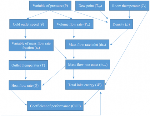
Figure 1. Mathematical method analysis diagram
2.2 Taguchi method
Taguchi developed a special orthogonal array design to study all parameter spaces with only minimum experiments. The Taguchi method uses a measure of performance statistics called the [S/N] ratio [14]. This method is used to reduce the number of experiments needed to achieve the goal depending on various parameters [15].
The [S/N] ratio is used to measure the characteristic quality deviating from the desired value. There are three categories in the signal to ratio analysis, namely [14]:
larger is better,
$\frac{S}{N}ratio(\eta )=-10\times {{\log }_{10}}\frac{1}{n}\sum\nolimits_{i=1}^{n}{\frac{1}{y_{1}^{2}}}$ (13)
nominal is best,
$\frac{S}{N}ratio(\eta )=-10\times {{\log }_{10}}\sum\nolimits_{i=1}^{n}{\frac{1}{n}}\frac{{{\mu }^{2}}}{{{\sigma }^{2}}}$ (14)
smaller is better,
$\frac{S}{N}ratio(\eta )=-10\times {{\log }_{10}}\sum\nolimits_{i=1}^{n}{y_{1}^{2}}$ (15)
Techniques of Analysis of variance (ANOVA) is used to test the adequacy of the model. This method is very useful to reveal the level of significance of the influence of factors or factors of interaction on a particular response. This separates the total variability of responses into the contributions given by each parameter and error [16].
$S{{S}_{Tot}}=S{{S}_{F}}+S{{S}_{e}}$ (16)
where,
$S{{S}_{Tot}}=\sum\nolimits_{j=1}^{p}{({{\gamma }_{j}}}-{{\gamma }_{m}})$ (17)
The mean square deviation in the ANOVA table is defined as [16]:
$MS=\frac{SS}{DF}$ (18)
The F-value of the Fisher ratio (variance ratio) is defined as:
$F=\frac{M{{S}_{t}}}{M{{S}_{et}}}$ (19)
The contribution of each factor is calculated by the following formula [14]:
$C\%=\frac{S_A}{S_z}$(20)
where,
${{S}_{z}}={{S}_{A}}+{{S}_{B}}+{{S}_{C}}$ (21)
In the last step of Taguchi's analysis, a data confirmation is performed to verify the most optimal parameters [16].
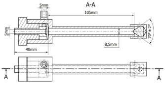
This study uses a type 1 vortex tube which uses no forced cooling and a type 2 which uses forced cooling on the heat tube. The dimensions of this tool are as follows: Din 5mm, Doutc 5mm Douth 8.5mm, Ltubec 40mm, Ltubeh 105mm, αplug 70 ±2o, and Ng 4. The size of the generator specifications is shown in Figure 4.
Figure 2. Dimension of vortex tube type 1
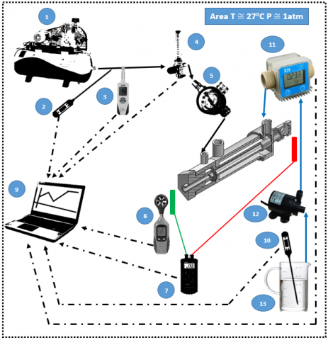
In Vortex tube type 1 forced cooling is developed by adding a tube that covers the hot tube. The material is made of PVC. Furthermore, in the tube flowed aquades (H2O) with contraflow flow direction and flow velocity 7 liters/minute. The incoming water temperature is controlled at 27 oC.
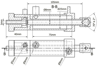
Figure 3. Dimension of vortex tube type 2
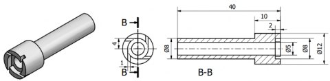
Figure 4. Size of generator specifications
Tests were carried out in Tr 27 oC conditions. The variables used are εcn 30 %, 40 %, 50 %, 60 %, and 70 % and pressure 0.5 bar, 1.0 bar, and 1.5 bar. In each of these variables, data was taken four times randomly with a duration interval of at least 5 seconds.
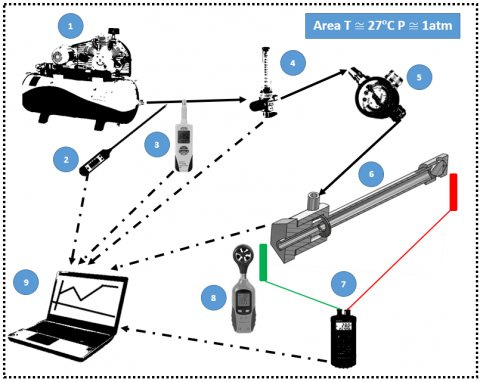
The series of experimental device for vortex tube type 1 is shown in Figure 5. The series of experimental tool for vortex tube type 2 shown in Figure 6.
Figure 5. Experiment series of vortex tube type 1
Figure 6. Experiment series of vortex tube type 2
Table 1. Information on Figures 5 and 6
|
No |
Name |
Function |
Unit (Symbol) |
|
1 |
Compressor |
Pressurized air supply |
- |
|
2 |
Digital Thermometer |
Measuring the temperature of the air inlet |
oCelcius (${{T}_{in}}$) |
|
3 |
Dew point Meter |
Measuring the inlet air dew point |
oCelcius ($T{{d}}$) |
|
4 |
Flow meter |
Measuring air flow |
Liter/min |
|
5 |
Pressure Gauge |
Measuring inlet air pressure |
Bar (P) |
|
6 |
Vortex tube |
Test instrument |
- |
|
7 |
Thermocouple |
Measuring hot and cold outlet air temperature |
oCelcius (Tc) and (Th) |
|
8 |
Anemometer |
Measuring the speed of cold outlet air |
meter/sec $({{v}_{\max }})$ and $({{v}_{n}})$ |
|
9 |
Computer |
Processing observation data from each measuring instrument |
- |
|
10 |
Digital Thermometer |
Measuring water temperature |
oCelcious |
|
11 |
Flow meter (water) |
Measuring water discharge |
Liter/min |
|
12 |
Pump |
pumping cooling water |
- |
|
13 |
Vessel |
Cooling water container |
- |
4.1 Presentation of experimental data
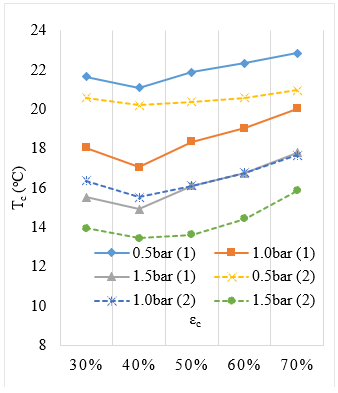
The experimental results of cold outlet temperature data and COPref of vortex tube are presented in the following diagram:
Figure 7. Cold temperature chart
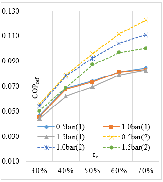
Figure 8. COPref chart
Cold temperature data presented in Figure 7 shows the tendency for the 40 % fraction to be the best. Higher pressure results in lower temperature of the cold outlet. Hamdan which has performed an experiment with different dimensions and forms of vortex tube also found for the pressure at 2bar, 3bar, and 4bar [7]. However an anomaly was found at 5bar pressure. The forced cooling on the heat tube affects the decreasing of temperature produced. These results are in accordance with the results of Eimsa's research in which cooling the heat tube by flowing water on the surface can reduce the temperature of the cold tank [2].
Based on Figure 8, it is found that the increasing cold fraction (εc) produces a better COPref. These results are also in accordance with Aydın's research with vortex tube dimensions and different generator forms found that cold fractions (20 % to 80 %) the greater the yield of COPref the better [1]. In this experiment, higher pressure produces lower COPref. The forced cooling treatment produces a better COPref. Eimsa by measuring isotropic efficiency found that cooling the surface of a hot tube by flowing water can improve its efficiency value [2].
4.2 Data reduction
For processing data with the Taguchi method, data reduction is done on the fraction factor to three levels that produce the best value. The cold temperature data that is produced smaller is the best and the COPref data the larger is the best. The selected data reduction is as follows:
Table 2. Reduction of cold temperature average data
|
Tube Type (TT) Natural Cooling (1) |
|||
|
Fraction (εc) |
Pressure (P) (bar) |
||
|
0.5 (1) |
1.0 (2) |
1.5 (3) |
|
|
30%(1) |
21.65 |
18.05 |
15.525 |
|
40%(2) |
21.1 |
17.05 |
14.925 |
|
50%(3) |
21.9 |
18.35 |
16.125 |
|
Tube Type (TT) Forc Cooling (2) |
|||
|
Fraction (εc) |
Pressure (P) (bar) |
||
|
0.5 (1) |
1.0 (2) |
1.5 (3) |
|
|
30%(1) |
20.600 |
16.375 |
13.950 |
|
40%(2) |
20.200 |
15.525 |
13.450 |
|
50%(3) |
20.400 |
16.125 |
13.625 |
Table 3. Reduction of COPref data
|
Tube Type (TT) Natural Cooling (1) |
|||
|
Fraction (εc) |
Pressure (P) (bar) |
||
|
0.5 (1) |
1.0 (2) |
1.5 (3) |
|
|
40%(1) |
-0.074 |
-0.074 |
-0.070 |
|
60%(2) |
-0.081 |
-0.081 |
-0.079 |
|
70%(3) |
-0.085 |
-0.083 |
-0.083 |
|
Tube Type (TT) Force Cooling (2) |
|||
|
Fraction (εc) |
Pressure (P) (bar) |
||
|
0.5 (1) |
1.0 (2) |
1.5 (3) |
|
|
40%(1) |
-0.096 |
-0.093 |
-0.087 |
|
60%(2) |
-0.112 |
-0.104 |
-0.097 |
|
70%(3) |
-0.123 |
-0.111 |
-0.100 |
4.3 Determining the orthogonal matrix
The orthogonal matrix is determined using statistical software Minitab 18. The orthogonal matrices used are L36 (21 32), where:
L : Latin square design,
36 : number of lines or experiments,
21 : one-factor column for two level, and
32 : two-factor column for three level.
4.4 Calculating the ratio of [S/N]
The data obtained from the experimental results are processed into the form of [S/N] ratio to determine the factors that influence the temperature of the vortex tube cold outlet. The [S/N] Signal-to-noise formula used for the cold temperature produced the smaller is better with equation (15), and for the COPref the larger is better with equation (13).
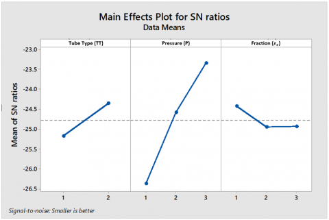
The most decisive parameter for vortex tube performance results for cold temperature show in Figure 9 and Table 5. The most determining parameters for the least related are pressure, tube type, and fraction. The value of cold temperature based on the calculation of [S/N] ratio is reached on the factor of tube type 2 (forced cooling), pressure 3 (1.5 bar) and fraction 1 (30 %).
Table 4. [S/N] Rasio Ortogonal Matriks L36 (21×32)
|
Exsperiment Number |
Coloum Number |
[S/N] Rasio |
|||
|
1 (TT) |
2 (P) |
3 (εc) |
Tc |
COPref |
|
|
1 |
1 |
1 |
1 |
-26.709 |
-22.587 |
|
2 |
1 |
2 |
2 |
-24.634 |
-21.814 |
|
3 |
1 |
3 |
3 |
-24.150 |
-21.638 |
|
4 |
1 |
1 |
1 |
-26.709 |
-22.587 |
|
5 |
1 |
2 |
2 |
-24.634 |
-21.814 |
|
6 |
1 |
3 |
3 |
-24.150 |
-21.638 |
|
7 |
1 |
1 |
1 |
-26.709 |
-22.587 |
|
8 |
1 |
2 |
2 |
-24.634 |
-21.814 |
|
9 |
1 |
3 |
3 |
-24.150 |
-21.638 |
|
10 |
1 |
1 |
1 |
-26.709 |
-22.587 |
|
11 |
1 |
2 |
2 |
-24.634 |
-21.814 |
|
12 |
1 |
3 |
3 |
-24.150 |
-21.638 |
|
13 |
1 |
1 |
2 |
-26.486 |
-21.805 |
|
14 |
1 |
2 |
3 |
-25.273 |
-21.612 |
|
15 |
1 |
3 |
1 |
-23.821 |
-23.107 |
|
16 |
1 |
1 |
2 |
-26.486 |
-21.805 |
|
17 |
1 |
2 |
3 |
-25.273 |
-21.612 |
|
18 |
1 |
3 |
1 |
-23.821 |
-23.107 |
|
19 |
2 |
1 |
2 |
-26.107 |
-19.031 |
|
20 |
2 |
2 |
3 |
-24.150 |
-19.628 |
|
21 |
2 |
3 |
1 |
-22.891 |
-21.197 |
|
22 |
2 |
1 |
2 |
-26.107 |
-19.031 |
|
23 |
2 |
2 |
3 |
-24.150 |
-19.090 |
|
24 |
2 |
3 |
1 |
-22.891 |
-21.197 |
|
25 |
2 |
1 |
3 |
-26.193 |
-18.216 |
|
26 |
2 |
2 |
1 |
-24.284 |
-20.677 |
|
27 |
2 |
3 |
2 |
-22.574 |
-20.279 |
|
28 |
2 |
1 |
3 |
-26.193 |
-18.216 |
|
29 |
2 |
2 |
1 |
-24.284 |
-20.677 |
|
30 |
2 |
3 |
2 |
-22.574 |
-20.279 |
|
31 |
2 |
1 |
3 |
-26.193 |
-18.216 |
|
32 |
2 |
2 |
1 |
-24.284 |
-20.677 |
|
33 |
2 |
3 |
2 |
-22.574 |
-20.279 |
|
34 |
2 |
1 |
3 |
-26.193 |
-18.216 |
|
35 |
2 |
2 |
1 |
-24.284 |
-20.677 |
|
36 |
2 |
3 |
2 |
-22.574 |
-20.279 |
Figure 9. Main effects plot for [S/N] ratio for cold temperature
Table 5. Response table for signal to noise ratios for cold temperature
|
Level |
Tube Type (TT) |
Pressure (P) |
Fraction (εc) |
|
1 |
-25.18 |
-26.37 |
-24.43 |
|
2 |
-24.37 |
-24.59 |
-24.95 |
|
3 |
-23.36 |
-24.94 |
|
|
Delta |
0.81 |
3.01 |
0.52 |
|
Rank |
2 |
1 |
3 |
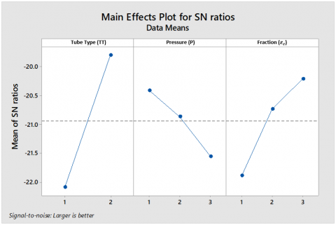
The parameters that have the most influence on COPref are shown in Figure 10 and Table 6. The parameters that most influence COPref from the most influential are type of tube, fraction, and pressure. The optimum COPref is achieved in tube type 2 (force cooling), pressure 1 (0.5 bar) and fraction 3 (70 %).
Figure 10. Main effects plot for [S/N] Ratio for COPref
Table 6. Response table for signal to noise ratios for COPref
|
Level |
Tube Type (TT) |
Pressure (P) |
Fraction (εc) |
|
1 |
-22.09 |
-20.41 |
-21.89 |
|
2 |
-19.79 |
-20.87 |
-20.73 |
|
3 |
-21.56 |
-20.21 |
|
|
Delta |
2.30 |
1.15 |
1.68 |
|
Rank |
1 |
3 |
2 |
4.5 ANOVA test
The ANOVA results for the [S/N] ratio were obtained using Minitab 18 statistical software as shown in Table 7 for cold temperatures, and Table 8 for COPref. The p-value shown in the ANOVA table shows the significance of each variable in the results. Factors are said to have a significant effect if the p-value is <0.05 [14-15]. In the table all p-values are 0, so all factors have a significant effect on cold temperature and COPref.
The F-test concept states that the higher the F-value, the more significant the factor is [15]. The results show that the order of influence for each factor for the ANOVA test whit the [S/N] ratio test is the same.
Table 7. Analysis of variance cold temperature
|
Source |
DF |
Adj SS |
Adj MS |
F-Value |
P-Value |
|
Tube Type |
1 |
21.468 |
21.468 |
401.48 |
0.000 |
|
Pressure |
2 |
232.588 |
116.294 |
2174.85 |
0.000 |
|
Fraction |
2 |
4.633 |
2.317 |
43.33 |
0.000 |
|
Error |
30 |
1.604 |
0.053 |
||
|
Lack-of-Fit |
6 |
1.604 |
0.267 |
* |
* |
|
Pure Error |
24 |
0.000 |
0.000 |
||
|
Total |
35 |
260.294 |
Table 8. Analysis of variance COPref
|
Source |
DF |
Adj SS |
Adj MS |
F-value |
P-value |
|
Tube Type |
1 |
0.005391 |
0.005391 |
522.59 |
0.000 |
|
Pressure |
2 |
0.000876 |
0.000438 |
42.46 |
0.000 |
|
Fraction |
2 |
0.002072 |
0.001036 |
100.42 |
0.000 |
|
Error |
30 |
0.000309 |
0.000010 |
||
|
Lack-of-Fit |
6 |
0.000287 |
0.000048 |
51.52 |
0.000 |
|
Pure Error |
24 |
0.000022 |
0.000001 |
||
|
Total |
35 |
0.008648 |
Equations (20) and (21) are utilized to find out how much the contribution of each factor is used on. The magnitude of the contribution of each factor is shown in the following Table 9:
Table 9. Contributions of each factor
|
Factor |
Response |
|
|
Cold Temperature |
COPref |
|
|
Tube Tipe |
8.25% |
62.34% |
|
Pressure |
89.36% |
10.13% |
|
Fraction |
1.78% |
23.96% |
|
Error |
0.62% |
3.57% |
|
Lack-of-Fit |
0.62% |
3.32% |
|
Pure Error |
0.00% |
0.25% |
|
Total |
100% |
100% |
4.6 Regression analysis
The regression equation is used to determine the value of the predictive response of each factor tested. To get the regression equation, Minitab 18 statistical software is used. The regression equation for cold temperatures Tc and COPref is as follows:
$R{{T}_{c}}=17.5194+0.7722T{{T}_{1}}-0.7722T{{T}_{2}}+\\ 3.3806{{P}_{1}}-0.6319{{P}_{2}}-2.7486{{P}_{3}}+\\0.0681{{F}_{1}}-0.4694{{F}_{2}}+0.4014{{F}_{3}}$ (22)
$RCO{{P}_{ref}}=0.091198-0.012237T{{T}_{1}}+0.012237T{{T}_{2}}\\0.006656{{P}_{1}}-0.001517{{P}_{2}}-0.005139{{P}_{3}}-\\0.009439{{F}_{1}}+0.000303{{F}_{2}}+0.009136{{F}_{3}}$ (23)
where,
P = pressure factor
F = fraction factor
TT = tube type factor
The regression equation above does not apply to all factor variables on vortex tube. This equation applies only to the factors and levels specified in this analysis.
4.7 Prediction of optimal value
Based on the value of [S/N] ratio and regression equation 22 and 23, the optimal predictive value is obtained:
${{T}_{c\_op}}=17.5194-0.7722~T{{T}_{\text{2}}}-~2.7486~{{P}_{\text{3}}}+~0.0681~{{F}_{\text{1}}}\\{{T}_{c\_op}}=17.5194-0.7722-2.7486+0.0681\\{{T}_{c\_op}}=14.07℃$ (24)
$CO{{P}_{ref\_op}}=0.091198+0.012237T{{T}_{\text{2}}}+\\ 0.006656{{P}_{\text{1}}}+0.009136{{F}_{\text{3}}}\\ CO{{P}_{ref\_op}}=0.091198+0.012237+0.006656+0.009136\\ CO{{P}_{ref\_op}}=0.119227$ (25)
4.8 Data confirmation
Data confirmation is performed by comparing the results of predictions with the experimental results presented in Table 10 below:
Table 10. Data Confirmation
|
Response |
Experiment |
Prediction |
Error (%) |
||
|
Level Factor |
Value |
Level Factor |
Value |
||
|
Cold Temperature |
TT2;P3;F2 |
13.45 |
TT2;P3;F1 |
14.07 |
4.61% |
|
COPref |
TT2;P1;F3 |
0.123 |
TT2;P1;F3 |
0.119 |
3.09% |
Based on Table 10 the level of error using the Taguchi method to predict the optimum value is 4.61 % for predictions of cold temperatures and 3.09 % for prediction of COPref.
It can be concluded that the optimization of vortex tube performance on parameters of tube type, pressure, and mass fraction with the Taguchi method are:
Based on the conclusions, it is known how the influence of tube type, pressure and fraction, so that this research can be a reference for the next research about optimization of vortex tube performance. The Taguchi method will be more accurate if use more number of level on each factor. In this study, the number of levels on each factor is small so that for further research to obtain the optimization of vortex tube performance with increasingly accurate results is done by increasing the number of levels in the pressure factor and fraction. In order for testing experiments to continue with effort, cost and time that is cheap, the level of factor is determined by referring to the most optimal point in this study.
The testing of the Taguchi method to measure the influence of tube types to the performance of vortex tubes in this study has only differentiated which ones have the most optimal performance. The results showed that the vortex tube with the type of forced cooling tube produced the most optimal performance. Based on these findings, the potential for optimizing the performance of vortex tube for further research is the engineering of forced cooling on the surface of the heat tube and the engineering of the heat flow.
|
COP |
coefficient of performance refrigeration |
|
$\dot{Q}$ |
heat flow |
|
$\dot{W}$ |
total energy |
|
$\dot{m}$ |
mass flow rate |
|
Cp |
heat capacity |
|
T |
Temperatur |
|
$\dot{V}$ |
volume flow rate |
|
Es |
saturation vapor pressure |
|
C |
coefficient |
|
eso |
Herman Wobus constant (6.1078) |
|
P |
air pressure |
|
Pv |
pressure of water vapor |
|
Es |
saturation vapor pressure |
|
Td |
dew point temperature |
|
Pv |
water vapor pressure |
|
R |
universal gas constan
|
|
$\vec{v}$ |
air velocity |
|
SS |
squared deviations number |
|
$\gamma$ |
average response |
|
MS |
mean square deviation in the ANOVA table |
|
DF |
degre of fredom |
|
C% |
contribution of each factor |
|
S |
each factor |
Greek symbols
|
$\rho$ |
density |
|
$\varepsilon$ |
fraction |
Subscripts
|
ref |
refrigeration |
|
c |
cold |
|
outc |
cold temperatures come out |
|
outh |
hot temperatures come out |
|
in |
inlet |
|
cn |
cold outlet variable to n |
|
c max |
cold outlet maximum conditions |
|
Tot |
total number |
|
F |
beacause of each other |
|
E |
due to error |
|
j |
for the jth experiment |
|
m |
for all experimental conditions |
|
t |
MS for a term |
|
et |
MS for the error term |
|
Z |
total Sum |
|
A, B, C |
each vaktor to A, B, C,. . . |
|
op |
optimal predictive |
[1] Aydin, O., Markal, B., Avci, M. (2010). A new vortex generator geometry for a counter-flow RanqueeHilsch vortex tube. Applied Thermal Engineering, 30(16): 2505-2511. https://doi.org/10.1016/j.applthermaleng.2010.06.024
[2] Eiamsa-ard, S., Wongcharee, K., Promvonge, P. (2010). Experimental investigation on energy separation in a counter-flow Ranque–Hilsch vortex tube: Effect of cooling a hot tube. International Communications in Heat and Mass Transfer, 37(2): 156–162. https://doi.org/10.1016/j.icheatmasstransfer.2009.09.013
[3] Attalla, M., Ahmed, H., Salem Ahmed, M., AboEl-Wafa, A. (2017). Experimental investigation for thermal performance of series and parallel Ranque-Hilsch vortex tube systems. Applied Thermal Engineering, 123: 327-339. https://doi.org/10.1016/j.applthermaleng.2017.05.084
[4] Alizadeh, M. (2018). Three dimensional numerical (3D CFD) study of effect of pressure-outlet and pressure-far-field boundary conditions on heat transfer predictions inside vortex tube. Progress in Solar Energy and Engineering Systems, 2(1): 21-25.
[5] Sadeghiazad, M.B.M. (2017). Experimental and numerical study on the effect of the convergence angle, injection pressure and injection number on thermal performance of straight vortex tube. International Journal of Heat and Technology, 35(3): 651-656. https://doi.org/10.18280/ijht.350324
[6] Sadeghiazad, M.B.M. (2017). Experimental study on thermal performance of double circuit vortex tube (DCVT) - Effect of heat transfer controller angle. International Journal of Heat and Technology, 35(3): 668-672. https://doi.org/10.18280/ijht.350327
[7] Hamdan, M.O., Al-Omari, S.A.B., Oweime, A.S. (2018). Experimental study of vortex tube energy separation under different tube design. Experimental Thermal and Fluid Scienc, 91: 306-311. https://doi.org/10.1016/j.expthermflusci.2017.10.034
[8] Pinar, A.M., Uluer, O., Kırmaci, V. (2009). Optimization of counter flow Ranque–Hilsch vortex tube performance using Taguchi method. International journal of refrigeration, 32(6): 1487-1494. https://doi.org/10.1016/j.ijrefrig.2009.02.018
[9] Yallamati, A., Vinjavarapu, S., Ashok, K.N. (2018). Using Taguchi method & response surface methodology for examination of surface roughness. Modelling Measurement and Control B, 87(1): 42-54.
[10] Suresh Kumar, G., Padmanabhan, G., Dattatreya Sarma, B. (2014). Optimizing the temperature of hot outlet air of vortex tube using Taguchi method. Procedia Engineering, 97: 828-836. https://doi.org/10.1016/j.proeng.2014.12.357
[11] Thøgersen, M.L. (2005). Modelling of the variation of air density with altitude through pressure, humidity and temperature. EMD International A/S, Niels Jernesvej, Aalborg, USA.
[12] Gao, O. (2005). Experimental Study on the Ranque-Hilsch Vortex Tube. Technische Universiteit Eindhoven, Australia.
[13] Çengel, Y.A., Cimbala, Y.M. (2014). Fluid Mechanics: Fundamentals and Applications, Third Edition. The Mcgraw-Hill Companies Inc, New York, USA.
[14] Derdour, F.Z., Kezzar, M., Bennis, O., Lakhdar, K. (2018). The optimization of the operational parameters of a rotary percussive drilling machine using the Taguchi method. World Journal of Engineering, 15(5): 62-69. https://doi.org/10.1108/WJE-03-2017-0067
[15] Zade, S.K., Suresh, B.V., Sai, S.K.V. (2018). Effect of nanoclay, glass fiber volume and orientation on tensile strength of epoxy-glass composite and optimization using Taguchi method. World Journal of Engineering, 15(1): 312-320. https://doi.org/10.1108/WJE-08-2017-0286
[16] Sreeraj, P., Kannan, T., Subhasis, M. (2014). Analysis of flux cored arc welding process parameters by hybrid Taguchi approach. World Journal of Engineering, 11(6): 575-588.