Anwar Saeed | Zahir Shah* | Abdullah Dawar | Saeed Islam | Waris Khan | Muhammad Idrees
© 2019 IIETA. This article is published by IIETA and is licensed under the CC BY 4.0 license (http://creativecommons.org/licenses/by/4.0/).
OPEN ACCESS
The greatest endowment of present-day science is nanofluid. The nanofluid can ready to move unreservedly through smaller scale channels with the spreading of nanoparticles. Because of improved convection between the base fluid surfaces and nanoparticles, the nanosuspensions express high warm conductivity. Additionally, the advantages of suspending nanoparticles in base liquids are expanded warmth limit, surface zone, successful warm conductivity, impact, and collaboration among particles. The point of this examination is to review the imaginative origination of entropy generation in the nanoparticles of single and multi-walled carbon nanotubes are suspended in the four disparate. Kerosene oil is taken as based nanofluids in view of its novel consideration because of their propelled warm conductivities, selective highlights, and applications. The leading equations have been converted to differential equations with the help of suitable variables. the homotopic approach has been utilized to solve the modeled problem. The impact of physical factors are discused in details.
entropy generation, SWCNTs and MWCNTs, rotating system, thermal radiation, HAM
Entropy is turmoil of a framework and encompassing. It happens when heat transmission happens, in light of the fact that some extra developments happen when it moves. For instance, sub-atomic vibration, and grinding, relocations of particles, active vitality, turn developments and so on. Because of which loss of valuable warmth happens and in this way radiation can't transmit completely into work. Disarray in a framework and encompassing made because of these extra developments. For this minute tumult results in naturally visible dimension which happens in view of some superfluous irreversibility’s. The Bejan [1] formulated the entropy generation rate. Sarojamma et al. [2] investigated the entropy generation in a thin film flow over a stretching sheet. Soomro et al. [3] have as of late analyzed numerically the entropy generation in MHD water-based CNTs. Mansour et al. [4] have been examined numerically the entropy generation rate in a laminar viscous flow in a roundabout flow and have thought that the entropy generation rate is high close to the divider and persistently diminishes along the sweep far from the outside of the pipe. Over a penetrable extending surface Rashidi at al. [5] have inspected the entropy generation for stagnation point flow in a permeable medium. The other related investigation about the entropy generation can be seen in [6-8].
The study of heat transfer flow is significant in numerous engineering applications, for instance, the design of thrust bearing, drag reduction, transpiration cooling, radial diffusers and thermal recovery of oil. Heat transfer has a vital role in handling and processing of non-Newtonian mixtures. In recent years, CNTs attained more interest for scientists and researchers because of the wide range applications in several industrial and engineering processes [9-15].
Choi [16] investigates nanofluid first time. Nanofluid scientific model was set up by Boungiorno [17]. The nature of nanoparticles and shape of nanoparticles are significant aspects to improve the thermal conductivity of working fluids are cited in [18-21]. They considered five shapes of nanoparticles and found that all the five different shape of nanoparticles increase the heat transmission characteristics. In a rotating system along with magnetic field, Sheikholeslami et al. [22] discussed the nanofluid flow and heat transmission. The learning of magnetic properties of electrically conducting fluids is known as magnetohydrodynamics (MHD) [23]. Haq et al. [24] were studied CNTs in cylinders with MHD. Abro et al. [25] analytically studied MHD Jeffery fluid under the impact of thermal radiation. The others related works can be studied Khan [26-31]. Dawar et al. [32] examined Eyring–Powell fluid flow under the impact of thermal radiation over a porous medium. The recent analysis of nanofluid with modern application can be seen in the research of [33-37]. The micro rotation effect on MHD Nanofluid was studied by Shah et al. [38- 41].
The foremost aim of this research is the investigation of numerical simulation of nanofluid flow through a permeable space. Working fluid is Kerosene Oil based nanofluid. Non-Darcy model was utilized to employ porous terms in momentum equations. Radiation effect has been reported for various shapes of nanoparticles. Impacts of, radiation parameter and magnetic force, on nanofluid behavior were demonstrated. HAM approach has used.
To investigate the entropy generation in a two-dimensional nanoparticle of SWCNTs and MWCNTs based on (water, engine oil, ethylene glycol and kerosene oil) in a rotating parallel porous plate in the main focus of this research work. To get the solution of the modeled problem, the HAM [42-46] is applied.
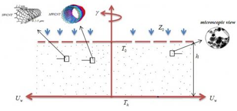
The CNTs nanofluid based on kerosene oil between two porous plates are considered. Plates are separated with distance h. The coordinate (x, y, z) system is taken with x-axis parallel, y-axis is taken vertical to the plate, and z is taken along xy plane. The plates are positioned at y=0, y=h and roating with constant angular velocity γ along y-asix. Both the plates are rotated in the same direction is denoted by γ>0, in opposite direction is denoted by γ<0, while γ=0 means the static case. The lower plate is moving quicker than the upper plate with velocity $\mathrm{U}_{w}=c \mathrm{x}(c>0)$.
Figure 1. Physical representation of the flow problem
After applying the problem assumptions basic equations are considered as
$\frac{\partial u}{\partial x}+\frac{\partial v}{\partial y}=0$ (1)
$\begin{align} & {{\rho }_{nf}}\left( u\frac{\partial u}{\partial x}+v\frac{\partial u}{\partial y}+2\gamma w \right)= \\ & -\frac{\partial {{P}^{*}}}{\partial x}+{{\mu }_{nf}}\left( \frac{{{\partial }^{2}}u}{\partial {{x}^{2}}}+\frac{{{\partial }^{2}}u}{\partial {{y}^{2}}} \right)-\frac{B}{K}u, \\ \end{align}$ (2)
${{\rho }_{nf}}\left( u\frac{\partial v}{\partial x}+v\frac{\partial v}{\partial y} \right)=-\frac{\partial {{P}^{*}}}{\partial y}+{{\mu }_{nf}}\left( \frac{{{\partial }^{2}}u}{\partial {{x}^{2}}}+\frac{{{\partial }^{2}}u}{\partial {{y}^{2}}} \right)$ (3)
$\begin{align} & {{\rho }_{nf}}\left( u\frac{\partial w}{\partial x}+v\frac{\partial w}{\partial y}-2\gamma u \right)= \\ & {{\mu }_{nf}}\left( \frac{{{\partial }^{2}}w}{\partial {{x}^{2}}}+\frac{{{\partial }^{2}}w}{\partial {{y}^{2}}} \right)+\frac{B}{K}w, \\ \end{align}$ (4)
where ${{P}^{*}}=P-\frac{{{\gamma }^{2}}{{x}^{2}}}{2},{{\sigma }_{nf}},{{\mu }_{nf}}$ indicate the modified pressure, electrical conductivity, and the dynamic viscosity of nanofluid respectively. In the absenteeism of $\frac{\partial {{P}^{*}}}{\partial z}$ represents the meshes cross flow beside z-axis. Mathematically, the phenomenon of heat transmission can be indicated as:
$u\frac{\partial T}{\partial x}+v\frac{\partial T}{\partial x}=\frac{{{k}_{nf}}}{{{(\rho c)}_{nf}}}\left( \frac{{{\partial }^{2}}T}{\partial {{x}^{2}}}+\frac{{{\partial }^{2}}T}{\partial {{y}^{2}}} \right)-\frac{\partial Qr}{\partial y}$ (5)
$\mathrm{T}, \alpha_{n f}=\frac{k_{n f}}{(\rho c)_{n f}}, Q r$ signifies the fluid temperature, thermal diffusivity and radiative heat flux respectively.
where Qr is:
$Q r=\frac{4 \sigma^{*}}{3 k} \frac{\partial \mathrm{T}^{4}}{\partial y}$ (6)
As $\mathrm{T}^{4}=4 \mathrm{T}_{h}^{3} \mathrm{T}-3 \mathrm{T}_{h}^{4}$ the equation (6) becomes:
$u \frac{\partial T}{\partial x}+v \frac{\partial T}{\partial y}=\frac{k_{n f}}{(\rho c)_{n f}}\left(1+\frac{16 \sigma^{*} \mathrm{T}_{h}^{3}}{3 k}\right) \frac{\partial^{2} T}{\partial y^{2}}$ (7)
The needed formulas are:
$\rho_{n f}=(1-\varphi)(\rho c)_{f}+\varphi(\rho c)_{C N T}$, $(\rho c)_{n f}=(1-\varphi) \rho_{f}+\varphi \rho_{C N T}, \mu_{n f}=\frac{\mu_{f}}{(1-\varphi)^{2.5}}$, $k_{n f}=\frac{1-\varphi+2 \varphi \frac{k_{C N T}}{k_{C N T}-k_{f}} \ln \frac{k_{C N T}+k_{f}}{2 k_{f}}}{1-\varphi+2 \varphi \frac{k_{f}}{k_{C N T}-k_{f}} \ln \frac{k_{C N T}+k_{f}}{2 k_{f}}} k_{f}$, $\sigma_{n f}=1+\frac{3\left(\frac{\sigma_{C N I}}{\sigma_{f}}-1\right) \varphi}{\left(\frac{\sigma_{C N T}}{\sigma_{f}}+2\right)-\left(\frac{\sigma_{C N T}}{\sigma_{f}}-1\right) \varphi} \sigma_{f}$ (8)
The boundary conditions are:
$u=U_{w}=c x, v=0, w=0, \mathrm{T}=\mathrm{T}_{h}$ at $y=0, u=0, \vec{v}=-Z_{0}, w=0, \mathrm{T}=\mathrm{T}_{0}$ at $y=h$ (9)
The similarity variables are:
$u=c x \frac{d f}{d \eta}, v=-c h f, w=\operatorname{cxg}, \theta=\frac{\mathrm{T}-\mathrm{T}_{0}}{\mathrm{T}_{h}-\mathrm{T}_{0}}, \eta=\frac{y}{h}$ (10)
The non-dimensional system of equations is:
$\frac{d^{4} f}{d \eta^{4}}-(1-\varphi)^{2.5}\left[\begin{array}{c}{(1-\varphi)} \\ {+\varphi \frac{\rho_{C N T}}{\rho_{f}}}\end{array}\right] R_{1}\left(\begin{array}{c}{\frac{d f}{d \eta} \frac{d^{2} f}{d \eta^{2}}} \\ {-f \frac{d^{3} f}{d \eta^{3}}}\end{array}\right)-(1-\varphi)^{2.5}\left[\begin{array}{c}{(1-\varphi)} \\ {+\varphi \frac{\rho_{C N T}}{\rho_{f}}}\end{array}\right] R_{2} \frac{d g}{d \eta}-\kappa \frac{d^{2} f}{d \eta^{2}}=0$ (11)
$\frac{d^{2} g}{d \eta^{2}}-(1-\varphi)^{2.5}\left[\begin{array}{c}{(1-\varphi)} \\ {+\varphi \frac{\rho_{C N T}}{\rho_{f}}}\end{array}\right] R_{1}\left(g \frac{d f}{d \eta}-f \frac{d g}{d \eta}\right)+2(1-\varphi)^{2.5}\left[\begin{array}{c}{(1-\varphi)} \\ {+\varphi \frac{\rho_{C N T}}{\rho_{f}}}\end{array}\right] R_{2} \frac{d f}{d \eta}+\kappa g=0$ (12)
$(1+R d) \frac{d^{2} \theta}{d \eta^{2}}+(1-\varphi)^{2.5}\left[(1-\varphi)+\varphi \frac{\rho_{C N T}}{\rho_{f}}\right] \frac{1}{\left(\frac{k_{n f}}{k_{f}}\right)} \operatorname{Pr} R_{1} f \frac{d \theta}{d \eta}=0$ (13)
The relevant boundary conditions are:
$\begin{align} & f=0,\frac{df}{d\eta }=1,g=0,\theta =1,\text{ at }\eta =0, \\ & f=s,\frac{df}{d\eta }=0,g=0,\theta =0,\text{ at }\eta =1. \\ \end{align}$ (14)
In equation (14), $s={}^{{{Z}_{0}}}/{}_{ch}$ is the suction and injection parameter.
In the above equations ${{R}_{1}}=\frac{c{{h}^{2}}}{{{\nu }_{f}}}$ is the Reynolds number, ${{R}_{2}}=\frac{\gamma {{h}^{2}}}{{{\nu }_{f}}}$ is the rotation parameter, $\Pr =\frac{{{\mu }_{f}}{{c}_{p}}}{{{k}_{f}}}$ is the Prandtl number, $R d=\frac{16 \sigma^{*} \mathrm{T}_{h}^{3}}{3 k k^{*}}$ is the thermal radiation parameter,
The skin friction and Nusselt number is defined as [22];
${{\tilde{C}}_{f}}=\frac{{{\mu }_{nf}}}{{{\mu }_{f}}}\frac{{{d}^{2}}f\left( 0 \right)}{d{{\eta }^{2}}},N{{u}_{x}}=-\frac{{{k}_{nf}}}{{{k}_{f}}}\left( 1+Rd \right)\frac{d\theta \left( 0 \right)}{d\eta }$ (15)
For a nanofluid, the local entropy rate ${{S}_{g.t}}$ per unit volume is:
$S_{g, t}^{\prime \prime \prime}=\frac{k_{n f}}{T_{0}^{2}}\left\{\begin{array}{l}{(\nabla T)^{2}} \\ {+\frac{16 \sigma^{*} T_{h}^{3}}{3 k k^{*}}(\nabla T)^{2}}\end{array}\right\}+\frac{\mu_{n f}}{T_{0}} \Phi+\frac{B}{T_{0}} u^{2}$ (16)
$S_{g, t}^{\prime \prime \prime}=\frac{k_{n f}}{T_{0}^{2}}\left\{\left(\begin{array}{c}{1+} \\ {\frac{16 \sigma^{*} T_{h}^{3}}{3 k}}\end{array}\right)(\nabla T)^{2}\right\}+\frac{\mu_{n f}}{T_{0}} \Phi+\frac{B}{T_{0}} u^{2}$ (17)
where $(\nabla T)=\frac{\partial \mathrm{T}}{\partial x}+\frac{\partial \mathrm{T}}{\partial y}$ and $\Phi$ is related to viscous dissipation.
In our case
$S_{g . t}^{\prime \prime \prime}=\frac{k_{n f}}{T_{0}^{2}}\left\{\left(1+\frac{16 \sigma^{*} T_{h}^{3}}{3 k k^{*}}\right)(\nabla T)^{2}\right\}+\frac{\mu_{n f}}{T_{0}}\left(\frac{\partial u}{\partial y}\right)^{2}+\frac{B}{K T_{0}} u^{2}$ (18)
The characteristic entropy generation rate ${{S}_{g.c}}$ is defined as:
$S_{g . c}^{\prime \prime \prime}=\frac{k_{n f}(\nabla \mathrm{T})^{2}}{T_{h}^{2} L^{2}}$ (19)
The entropy generation Ns is defined is:
$Ns=\frac{{{{{S}'''}}_{g.t}}}{{{{{S}'''}}_{g.c}}}$ (20)
To calculate the entropy generation Ns, using equations (18) and (19) to gather with (10) in equation (20), we obtain as:
$N_{S}=R_{1}\left\{\begin{array}{l}{(1+R d)\left(\frac{d \theta}{d \eta}\right)^{2}} \\ {+\frac{1}{(1-\varphi)^{2.5}}\left(\frac{B r}{\omega} \frac{d^{2} f}{d \eta^{2}}+\kappa^{2}\left(\frac{d f}{d \eta}\right)^{2}\right)}\end{array}\right\}$ (21)
where ${{R}_{1}}$ is the Reynolds number, Br is t the Brinkman number and $\omega$ is the non-dimensionless temperature whose expression are given by:
$R_{1}=\mathrm{T}_{h}^{2} L^{2}, \omega=\frac{\mathrm{T}_{h}-\mathrm{T}_{0}}{\mathrm{T}_{0}}, ? \mathrm{Br}=\frac{\mu_{f} U_{w}^{2}}{k_{n f}\left(\mathrm{T}_{h}-\mathrm{T}_{0}\right)}$ (22)
The Bejan number Be is defined as:
$B e=\frac{\frac{k_{n f}}{\mathrm{T}_{0}^{2}}\left(1+\frac{16 \sigma^{*} T_{h}^{3}}{3 k k^{*}}\right)\left(\frac{\partial \mathrm{T}}{\partial y}\right)^{2}}{\frac{\mu_{n f}}{\mathrm{T}_{0}}\left(\frac{\partial u}{\partial y}\right)^{2}+\frac{B}{K \mathrm{T}_{0}} u^{2}}$ (23)
$B e=\frac{R_{1}(1+R d)\left(\frac{d \theta}{d \eta}\right)^{2}}{R_{1}\left\{\frac{1}{(1-\varphi)^{25}}\left(\frac{B r}{\omega} \frac{d^{2} f}{d \eta^{2}}+\kappa^{2}\left(\frac{d f}{d \eta}\right)^{2}\right)\right\}}$ (24)
We use HAM [40-45] to solve Eqns. (11, 12, and 13) with (14) by the succeeding process.
The primary suppositions are chosen as follows:
$\overline{f}(\eta)=\eta+\frac{1}{2}(Q-1) \eta^{2}, \overline{\mathrm{g}}_{0}(\eta)=0, \overline{\theta}_{0}(\eta)=1-\eta$ (25)
The linear operators are chosen as ${{\text{L}}_{{\bar{f}}}}\text{,}{{\text{L}}_{{\bar{g}}}}\text{ and }{{\text{L}}_{{\bar{\theta }}}}$:
${{L}_{{\bar{f}}}}(\bar{f})=\bar{f}''',\text{ }{{\text{L}}_{{\bar{g}}}}\text{(\bar{g})=\bar{g} }\!\!'\!\!\text{ }\!\!'\!\!\text{ },\text{ }{{\text{L}}_{{\bar{\theta }}}}\text{(}\bar{\theta }\text{)=}\bar{{\theta }''}$ (26)
which have the succeeding properties:
${{L}_{{\bar{f}}}}({{t}_{1}}+{{t}_{2}}\eta +{{t}_{3}}{{\eta }^{2}})=0,\text{ }{{\text{L}}_{{\bar{g}}}}({{t}_{4}}+{{t}_{5}}\eta )=0,{{\text{L}}_{{\bar{\theta }}}}({{t}_{6}}+{{t}_{7}}\eta )=0$ (27)
where ${{t}_{i}}(i=1-7)$.
Non-linear operators ${{N}_{{\bar{f}}}},{{N}_{{\bar{g}}}}$ and ${{N}_{{\bar{\theta }}}}$ are indicated as:
$N_{\overline{f}}[\overline{f}(\eta ; \psi), \overline{g}(\eta ; \psi)]=\frac{d^{4} \overline{f}(\eta ; \psi)}{d \eta^{4}}$
$-(1-\varphi)^{2.5}\left[(1-\varphi)+\varphi \frac{\rho_{C N T}}{\rho_{f}}\right] R_{1}\left\{\frac{d \overline{f}(\eta ; \psi)}{d \eta} \frac{d^{2} \overline{f}(\eta ; \psi)}{d \eta^{2}}-\overline{f}(\xi ; \psi) \frac{d^{3} \overline{f}(\xi ; \psi)}{d \xi^{3}}\right\}$
$-(1-\varphi)^{2.5}\left[(1-\varphi)+\varphi \frac{\rho_{C N T}}{\rho_{f}}\right] R_{2} \frac{d \overline{g}(\eta ; \psi)}{d \eta}-\kappa \frac{d^{2} \overline{f}(\eta ; \psi)}{d \eta^{2}}$ (28)
$N_{\overline{g}}[\overline{f}(\eta ; \psi), \overline{g}(\eta ; \psi)]=\frac{d^{2} \overline{g}(\eta ; \psi)}{d \eta^{2}}$
$-(1-\varphi)^{2.5}\left[(1-\varphi)+\varphi \frac{\rho_{C N T}}{\rho_{f}}\right] R_{1}\left(\overline{g}(\eta ; \psi) \frac{d \overline{f}(\eta ; \psi)}{d \eta}-\overline{f}(\eta ; \psi) \frac{d \overline{g}(\eta ; \psi)}{d \eta}\right)$
$+2(1-\varphi)^{2.5}\left[(1-\varphi)+\varphi \frac{\rho_{C N T}}{\rho_{f}}\right] R_{2} \frac{d \overline{f}(\eta ; \psi)}{d \eta}+\kappa \overline{g}(\eta ; \psi)$ (29)
$N_{\overline{\theta}}[\overline{f}(\eta ; \psi), \overline{\theta}(\eta ; \psi)]=(1+R d) \frac{d^{2} \overline{\theta}(\eta ; \psi)}{d \eta^{2}}$
$+\left[(1-\varphi)+\varphi \frac{\left(\rho c_{p}\right)_{C N T}}{\left(\rho c_{p}\right)_{f}}\right] \frac{1}{\left(\frac{k_{n f}}{k_{f}}\right)} \operatorname{Pr} R_{1} \overline{f}(\eta, \psi) \frac{d \overline{\theta}(\eta ; \psi)}{d \eta}$ (30)
In organize to solve Eqns. (11, 12, and 13) are:
$(1-\psi ){{L}_{{\bar{f}}}}\left[ \bar{f}(\eta ;\psi )-{{{\bar{f}}}_{0}}(\eta ) \right]=\psi {{\hbar }_{{\bar{f}}}}{{N}_{{\bar{f}}}}\left[ \bar{f}(\eta ;\psi ),\bar{g}(\eta ;\psi ) \right]$ (31)
$(1-\psi ){{L}_{{\bar{g}}}}\left[ \bar{g}(\eta ;\psi )-{{{\bar{g}}}_{0}}(\eta ) \right]=\psi {{\hbar }_{{\bar{g}}}}{{N}_{{\bar{g}}}}\left[ \bar{f}(\eta ;\psi ),\bar{g}(\eta ;\psi ) \right]$ (32)
$(1-\psi ){{L}_{{\bar{\theta }}}}\left[ \bar{\theta }(\eta ;\psi )-{{{\bar{\theta }}}_{0}}(\eta ) \right]=\psi {{\hbar }_{{\bar{\theta }}}}{{N}_{{\bar{\theta }}}}\left[ \bar{f}(\eta ;\psi ),\bar{\theta }(\eta ;\psi ) \right]$ (33)
The equivalent boundary conditions are:
$\overline{f}\left.(\eta ; \psi)\right|_{\eta=0}=0,\left.\frac{\overline{f}(\eta ; \psi)}{d \eta}\right|_{\eta=0}=1, \overline{f}\left.(\eta ; \psi)\right|_{\eta=1}=s,\left.\frac{d \overline{f}(\eta ; \psi)}{\partial \eta}\right|_{\eta=1}=0,$
$\overline{g}\left.(\eta ; \psi)\right|_{\eta=0}=0, \overline{g}\left.(\eta ; \psi)\right|_{\eta=1}=0, \overline{\theta}\left.(\eta ; \psi)\right|_{\eta=0}=1, \overline{\theta}\left.(\eta ; \psi)\right|_{\eta=1}=0$ (34)
where $\psi \in [0,1]$ is the emerging parameter. In case of $\psi =0\text{ and }\psi =1$ we have:
$\begin{align} & \bar{f}(\eta ;0)={{{\bar{f}}}_{0}}(\eta )\text{, }\bar{f}(\eta ;1)=\bar{f}(\eta )\text{, } \\ & \text{\bar{g}}(\eta ;0)={{{\bar{g}}}_{0}}(\eta ),\text{ }~\text{\bar{g}}(\eta ;1)=\bar{g}(\eta ),~ \\ & \bar{\theta }(\eta ;0)={{{\bar{\theta }}}_{0}}(\eta ),~~~~~\bar{\theta }(\eta ;1)=\bar{\theta }(\eta ). \\ \end{align}$ (35)
Expanding $\overline{f}(\eta ; \psi), \overline{g}(\eta ; \psi)$ and $\overline{\theta}(\eta ; \psi)$ by Taylor’s series
$\overline{f}(\eta ; \psi)=\overline{f}_{0}(\eta)+\sum_{q=1}^{\infty} \overline{f}_{q}(\eta) \psi^{q}, \overline{g}(\eta ; \psi)=\overline{g}_{0}(\eta)+\sum_{q=1}^{\infty} \overline{g}_{q}(\eta) \psi^{q}, \overline{\theta}(\eta ; \psi)=\overline{\theta}_{0}(\eta)+\sum_{q=1}^{\infty} \overline{\theta}_{q}(\eta) \psi^{q}$ (36)
where
${{\bar{f}}_{q}}(\eta )={{\left. \frac{1}{q!}\frac{d\bar{f}(\eta ;\psi )}{d\eta } \right|}_{\psi =0}}\text{,}{{\text{\bar{g}}}_{q}}(\eta )={{\left. \frac{1}{q!}\frac{d\bar{g}(\eta ;\psi )}{d\eta } \right|}_{\psi =0}},\text{and }{{\bar{\theta }}_{q}}(\eta )={{\left. \frac{1}{q!}\frac{d\bar{\theta }(\eta ;\psi )}{d\eta } \right|}_{\psi =0}}$ (37)
As the series (36) converges at $\psi =1$, changing $\psi =1$ in (36), we get:
$\overline{f}(\eta)=\overline{f}_{0}(\eta)+\sum_{q=1}^{\infty} \overline{f}_{q}(\eta), \overline{g}(\eta)=\overline{g}_{0}(\eta)+\sum_{q=1}^{\infty} \overline{g}_{q}(\eta), \overline{\theta}(\eta)=\overline{\theta}_{0}(\eta)+\sum_{q=1}^{\infty} \overline{\theta}_{q}(\eta)$ (38)
The ${{q}^{th}}$-order problem gratifies the following:
${{L}_{{\bar{f}}}}\left[ {{{\bar{f}}}_{q}}(\eta )-{{\chi }_{q}}{{{\bar{f}}}_{q-1}}(\eta ) \right]={{\hbar }_{{\bar{f}}}}U_{q}^{{\bar{f}}}(\eta ),{{L}_{{\bar{g}}}}\left[ {{{\bar{g}}}_{q}}(\eta )-{{\chi }_{q}}{{{\bar{g}}}_{q-1}}(\eta ) \right]={{\hbar }_{{\bar{g}}}}U_{q}^{{\bar{g}}}(\eta ),{{L}_{{\bar{\theta }}}}\left[ {{{\bar{\theta }}}_{q}}(\eta )-{{\chi }_{q}}{{{\bar{\theta }}}_{q-1}}(\eta ) \right]={{\hbar }_{{\bar{\theta }}}}U_{q}^{{\bar{\theta }}}(\eta )$ (39)
The equivalent boundary conditions are:
$\overline{f}_{q}(0)=\overline{f}_{q}^{\prime}(0)=\overline{f}_{q}(1)=\overline{f}_{q}^{\prime}(1)=0, \overline{g}_{q}(0)=\overline{g}_{q}(1)=0, \overline{\theta}_{q}(0)=\overline{\theta}_{q}(1)=0$ (40)
Here
$U_{q}^{\overline{f}}(\eta)=\overline{f}_{q-1}^{i v}-R_{1}(1-\varphi)^{2.5}\left[(1-\varphi)+\varphi \frac{\rho_{C N T}}{\rho_{f}}\right]\left(\sum_{k=0}^{q-1} \overline{f}_{q-1-k}^{\prime} \overline{f}_{k}^{\prime \prime}-\sum_{k=0}^{q-1} \overline{f}_{q-1-k} \overline{f}_{k}^{\prime \prime \prime}\right)$
$-R_{2}(1-\varphi)^{2.5}\left[(1-\varphi)+\varphi \frac{\rho_{C N T}}{\rho_{f}}\right] \overline{g}_{q-1}-\kappa \overline{f}_{q-1}^{\prime \prime}$ (41)
$U_{q}^{\overline{g}}(\eta)=\overline{g}_{q-1}^{\prime \prime}-(1-\varphi)^{2.5}\left[(1-\varphi)+\varphi \frac{\rho_{C N T}}{\rho_{f}}\right] R_{1}\left(\sum_{k=0}^{q-1} \overline{g}_{q-1-k} \overline{f}_{k}^{\prime}-\sum_{k=0}^{q-1} \overline{f}_{q-1-k} \overline{g}_{k}^{\prime}\right)$
$+2(1-\varphi)^{2.5}\left[(1-\varphi)+\varphi \frac{\rho_{C N T}}{\rho_{f}}\right] R_{2} \overline{f}_{q-1}^{\prime}+\kappa \overline{g}_{q-1}$ (42)
$U_{q}^{\overline{\theta}}(\eta)=(1+R d) \overline{\theta}_{q-1}^{\prime \prime}+\left[(1-\varphi)+\varphi \frac{\left(\rho c_{p}\right)_{C N T}}{\left(\rho c_{p}\right)_{f}}\right] \frac{1}{\left(\frac{k_{n f}}{k_{f}}\right)} \operatorname{Pr} R_{1} \sum_{k=0}^{q-1} \overline{f}_{q-1-k} \overline{\theta}_{k}^{\prime \prime}$ (43)
where
$\chi_{q}=\left\{\begin{array}{ll}{0,} & {\text { if } \psi \leq 1} \\ {1,} & {\text { if } \psi>1}\end{array}\right.$
To investigate the flow and heat transfer performance for both SWCNTs and MWCNTs based on kerosene nanoliquids, consequences are schemed in Figures 2-22, telling the disparity in the velocities profiles (df/dη and g(η)), temperature profile θ(η), Entropy generation Ns and Bejan number Be within the circumscribed defined domain.
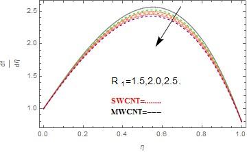
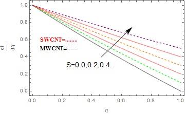
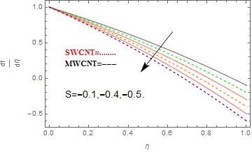
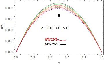
The impacts of embedded parameters on velocity function df/dη are displayed in Figures 2-11. Figure 2 displays the impact of (φ) on df/dη. The escalation in (φ) upsurges the df/dη. We have observed that MWCNTs has much greater increase in the velocity as compared to the SWCNTs. The impact of R1 on df/dη is depicted in Figure 3. The escalating values of R1 reducing the df/dη. This effect is due to the stretching of the plate. Figure 4 depicts the effect of R2 on df/dη. From Figure 4, we see that df/dη gives increasing behavior due to numerous rising values of R2. We have seen that the upper half of the plates gives more dominant variation to df/dη. The effect of $\kappa $ on df/dη shown in Figure 5. The rising in porosity parameter $\kappa $ rises the df/dη. The porous media plays an important role during the fluid flow phenomena. Actually, the porous media reduces the fluid velocity. Therefore, the increasing porous media reduces the velocity function. Figure 6 and 7 depict the effects of suction (s>0) and injection (s<0) parameters at the upper plate for df/dη. From Figure 6, we see that df/dη escalates with suction(s>0), that is df/dη increases with positive values of s. While from Figure 7, it is observed that df/dη diminishes with injection (s<0), that is df/dη reduces with negative values of s. It is fairly obvious that the presence of CNTs nanoparticles has improved df/dη, while df/dη upsurges further when (s>0) exists. But the reduction in df/dη is because of the fact that (s<0) engages the internal heat energy from the surface. The effect of φ on g(η) is depicted in Figure 8. The increasing φ increases the g(η). The MWCNTs has much greater increase in velocity function as compared to the SWCNTs is observed form here. Figure 9 is displayed to see the impact of R1 on g(η). The g(η) reduces with increasing in R1. The effect of R2 on g(η) is presented in Figure 10. From Figure 10, we see that the expanding estimations of R2 gives diminishing conduct in g(η). It can likewise be seen that the aggravation in g(η) is higher at the mode of the channel when contrasted with upper and lower surface of the channel. Figure 11 is plotted to see the effect of $\kappa $ on g(η). The porosity parameter has reverse impact on g(η), that is the g(η) diminishes with the heightening in $\kappa $.
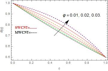
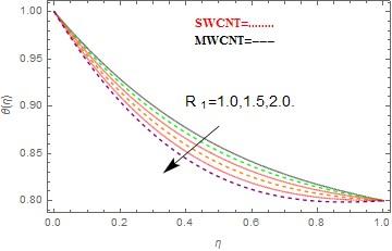
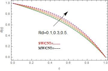
Figures 12-15 are plotted to see the effect of rising parameters on temperature function θ(η) for both SWCNTs and MWCNTs based on kerosene nanoliquids. Figure 12 is plotted to see the correlation between the SWCNTs and MWCNTs with the heightening estimations of φ. From Figure 12 we saw that there is unimportant dissimilarity in θ(η) with the heightening estimations of φ. We additionally have seen that the MWCNTs have nearly a lot more θ(η) noteworthy when contrasted with SWCNTs. Figure 13 depicts the effect of R1 on θ(η). The raising estimations of R1 shows heightening in θ(η) is appeared in Figure 13. As the separation from the surface heightens the θ(η) diminishes. Figure 14 is plotted to see the effect of Pr show on θ(η). From here we see that the raising estimations of shows decrease in θ(η). Physically, the nanofluids have an enormous warm diffusivity with little Pr, however this impact is revers for higher Pr, accordingly the temperature of fluid shows diminishing conduct. Figure 15 is plotted to see the effect of Rd on θ(η). Thermal radiation has driving principle in heat transmission when the coefficient of convection heat transmission is little. From here we see that the heightening estimations of Rd shows speeding up in θ(η).
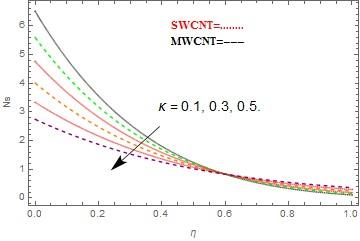
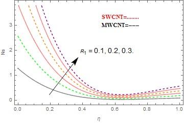
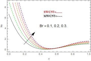
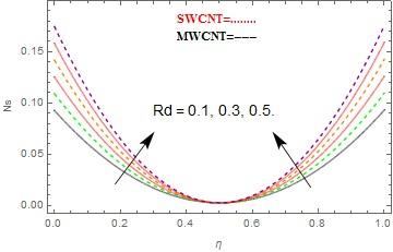
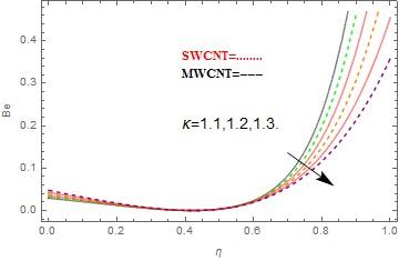
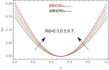
Figures 16-22 are plotted to see the impacts of developing parameters for both SWCNTs and MWCNTs based on kerosene nanoliquids on entropy generation Ns and Bejan number Be. For the most part, Ns is more for SWCNTs when contrasted with MWCNTs. Figures 16 demonstrates the effect of $\kappa $ on Ns. It is obvious from figure the assume that the heightening estimations of $\kappa $ shows diminishing conduct in Ns. Figure 17 shows the effect of Reynolds number R1 on Ns. From here we saw that with exceptionally little expanding in R1 the entropy generation raise all around rapidly, however at 0.4<ξ<0.6 a little expanding happens in Ns. It is because of extending of the lower plate. Figure 18 demonstrates the impact of Brinkman number Br on Ns. The Ns raises with the acceleration in Br. Furthermore, an expansion in Ns delivered by liquid rubbing and joule scattering happens with the heightening estimations of Br. Figure 19 demonstrates the impact of radiation parameter Rd on Ns. From the figure we see that at 0 <ξ< 0.5 and 0.5 <ξ< 1.0 the heightening estimations of Rd shows expanding conduct in Ns. Yet, at the mean position (i.e. ξ= 0.5) the thermal radiation has no impact on Ns. It is because of the extending of the lower plate. Figure 20 demonstrates the impact of $\kappa $ on Be. It is obvious from the assumes that the raising estimations of $\kappa $ shows diminishing conduct in Be. Figure 21 demonstrates the impact of Br on Be. Expanding Br gives heightening conduct in Be. Figure 22 demonstrates the impact of Rd on Be. From the figure we see that at 0 <ξ< 0.5 and 0.5 <ξ< 1.0 the expanding estimations of Rd show expanding conduct in Be, while at ξ= 0.5 the radiation parameter does not show expanding or diminishing conduct. It is because of the extending of the lower plate.
Figure 2. The plot of φ on $\frac{d f}{d \eta}$, when ${{R}_{1}}=0.5,{{R}_{2}}=0.6,s=0.8,\kappa =1.0$
Figure 3. The plot of ${{R}_{1}}$ on $\frac{df}{d\eta }$, when $\varphi =0.04,{{R}_{2}}=0.6,s=0.8,\kappa =1.0$
Figure 4. The plot of ${{R}_{2}}$ on $\frac{df}{d\eta }$, when $\varphi =0.04,{{R}_{1}}=0.5,s=0.8,\kappa =1.0$
Figure 5. The plot of $\kappa $ on $\frac{df}{d\eta }$, when $\varphi =0.04,{{R}_{1}}=0.5,{{R}_{2}}=0.6,s=0.8$
Figure 6. The plot of suction $\left( s>0 \right)$ on $\frac{df}{d\eta }$, when $\varphi =0.04,{{R}_{1}}=0.5,{{R}_{2}}=0.6,\kappa =1.0$
Figure 7. The plot of injection $\left( s<0 \right)$ on $\frac{df}{d\eta }$, when $\varphi =0.04,{{R}_{1}}=0.5,{{R}_{2}}=0.6,\kappa =1.0$
Figure 8. The plot of $\varphi $ on $g(\eta )$, when ${{R}_{1}}=0.5,{{R}_{2}}=0.6,\kappa =1.0$
Figure 9. The plot of ${{R}_{1}}$ on $g(\eta )$, when $\varphi =0.04,{{R}_{2}}=0.6,\kappa =1.0$
Figure 10. The plot of ${{R}_{2}}$ on $g(\eta )$, when $\varphi =0.04,{{R}_{1}}=0.5,\kappa =1.0$
Figure 11. The plot of $\kappa $ on $g(\eta )$, when $\varphi =0.04,{{R}_{1}}=0.5,{{R}_{2}}=0.6$
Figure 12. The plot of $\varphi $ on $\theta (\eta )$, when ${{R}_{1}}=0.5,\Pr =7.1,Rd=0.9$
Figure 13. The plot of ${{R}_{1}}$ on $\theta (\eta )$, when $\varphi =0.04,\Pr =7.1,Rd=0.9$
Figure 14. The plot of $\Pr $ on $\theta (\eta )$, when $\varphi =0.04,{{R}_{1}}=0.5,Rd=0.9$
Figure 15. The plot of $Rd$ on $\theta (\eta )$, when $\varphi =0.04,{{R}_{1}}=0.5,\Pr =7.1$
Figure 16. The plot of $\kappa $ on $Ns$, when $\varphi =0.04,Rd=0.9,\omega =0.5,Br=0.25,{{\operatorname{R}}_{1}}=1.0$
Figure 17. The plot of ${{\operatorname{R}}_{1}}$ on $Ns$, when $\varphi =0.04,Rd=0.9,\omega =0.5,Br=0.25,\kappa =1.0$
Figure 18. The plot of $Br$ on $Ns$, when $\varphi =0.04,Rd=0.9,\omega =0.5,\kappa =0.25,{{\operatorname{R}}_{1}}=1.0$
Figure 19. The plot of Rd on Ns, when $\varphi =0.04,{{\operatorname{R}}_{1}}=1.0,\omega =0.5,Br=0.5,\kappa =0.25$
Figure 20. The plot of $\kappa $ on Be, when $\varphi =0.04,Rd=0.9,\omega =0.5,Br=0.25$
Figure 21. The plot of Br on Be, when $\varphi =0.04,Rd=0.9,\omega =0.5,\kappa =0.25$
Figure 22. The plot of Rd on Be, when $\varphi =0.04,Br=0.25,\omega =0.5,\kappa =0.25$
Table 1. The numerical values of skin fraction when $\sigma =0.04$
|
${{R}_{1}}$ |
${{R}_{2}}$ |
s |
s |
${{\tilde{C}}_{f}}$ |
|
0.2 |
0.2 |
0.3 |
0.5 |
0.419391 |
|
0.4 |
|
|
|
0.418104 |
|
0.6 |
0.1 |
|
|
0.418885 |
|
|
0.3 |
|
|
0.418213 |
|
|
0.5 |
0.2 |
|
0.417078 |
|
|
|
0.6 |
|
0.468820 |
|
|
|
1.1 |
|
0.453513 |
|
|
|
1.4 |
-.5 |
0.427078 |
|
|
|
|
-.1 |
-3.821310 |
|
|
|
|
0.1 |
-1.152610 |
|
|
|
|
.5 |
-0.900993 |
Table 1 and 2 are conspired to see the impacts of various implanting parameters on C(~)f and Nux. From table 1, we see that the impact of R1 on skin portion. It is obvious from the table that at 0.1, the table shows expanding conduct to 0.3 however from 0.3 to 0.5, the table qualities show diminishing conduct. At the mode of the channel the C(~)f changes its conduct from raising to lessening. This is a direct result of extending of the lower plates. It is likewise obvious from the table that the rising estimations of R2 shows dropping conduct. The heightening estimations of $\kappa $ shows diminishing conduct in C(~)f. The expanding and diminishing estimations of suction/infusion parameter s shows two unique practices. The developing estimations of (s<0) presentations declining conduct and furthermore the rising estimations of (s>0) showcases swelling conduct in C(~)f. From table 2, we get that the swelling values of R1 and positive s (i.e. s>0) displays growing behavior in local Nusselt number Nux while R2, M and negative s (i.e. s < 0) displays declining behavior in local Nusselt number Nux. Tables 3-5 are conspired to think about the Physical properties of CNTs, thermo physical properties CNTs and nanofluids of some base liquids, Thermal conductivity (knf) of CNTs with various volume division (φ) individually.
Table 2. The numerical values of Nusselt number when $\sigma =0.04$
|
${{R}_{1}}$ |
${{R}_{2}}$ |
Pr |
Rd |
$\kappa $ |
s |
$N{{u}_{x}}$ |
|
0.2 |
0.3 |
7.1 |
0.1 |
0.3 |
0.5 |
-0.001840 |
|
0.4 |
|
|
|
|
|
-0.001938 |
|
0.6 |
0.3 |
|
|
|
|
-0.001937 |
|
|
0.5 |
|
|
|
|
-0.003874 |
|
|
0.7 |
7.2 |
|
|
|
-0.005689 |
|
|
|
7.3 |
|
|
|
-0.004149 |
|
|
|
7.4 |
0.2 |
|
|
-0.003649 |
|
|
|
|
1.1 |
|
|
-0.003449 |
|
|
|
|
2.1 |
0.1 |
|
-0.002689 |
|
|
|
|
|
0.2 |
|
-0.005650 |
|
|
|
|
|
0.3 |
|
-0.005628 |
|
|
|
|
|
1.3 |
-.5 |
-0.005610 |
|
|
|
|
|
|
-.1 |
-0.000400 |
|
|
|
|
|
|
0.1 |
-0.003186 |
|
|
|
|
|
|
.5 |
-0.003509 |
Entropy generation examination for the two-dimensional mixed convection flow of nanofluid based on kerosene over a porous extending sheet with suction/injection and radiative heat flux impacts are analyzed. SWCNTs and MWCNTs are utilized in this model. With the assistance of closeness factors, the arrangement of overseeing partial differential conditions is changed into ordinary differential conditions. The effects of implanted parameters are appeared. On the accomplished examination, the key comments are recorded beneath.
a. The velocity function df/dη escalates with the escalation in φ, R2 and suction parameter s, and reduces with the escalation in R1, $\kappa $ and injection parameter s.
b. The velocity function g(η) indicates acceleration conduct with heightening in φ and show decreasing conduct with heightening in, and R1, R2 and $\kappa $.
c. The temperature function θ(η) shows raising conduct with the acceleration in φ, and Rd shows diminishing conduct with the heightening in R1 and Pr.
d. The entropy generation Ns shows escalating behavior with the escalation Br. Also with a very small increase in R1 shows increasing behavior very quickly, while within the region 0.4<η<0.6, Re shows small increasing behavior. Rd shows increasing behavior in entropy generation Ns within the region 0<η<0.5 and 0.5<η≤<1.0, and has no effect at mean position (i.e. η=0.5).
e. The Bejan number Be shows increasing behavior with the increase in Br. Rd shows increasing behavior in Bejan number Be within the region 0<η<0.5 and 0.5<η≤<1.0, and has no effect at mean position (i.e. η=0.5).
[1] Bejan, A. (1995). Entropy Generation Minimization: The Method of Thermodynamic Optimization of Finite-size Systems and Finite-time Processes. CRC Press: Boca Raton, FL, USA.
[2] Sarojamma, G., Vajravelu, K., Sreelakshmi, K. (2017). A study on entropy generation on thin film flow over an unsteady stretching sheet under the influence of magnetic field, thermocapillarity, thermal radiation and internal heat generation/absorption. Communications in Numerical Analysis, 2017(2): 141-156. https://doi.org/10.5899/2017/cna-00319
[3] Soomro, F.A., Haq, R., Khan, Z.H., Zhang, Q. (2017). Numerical study of entropy generation in MHD water-based carbon nanotubes along an inclined permeable surface. European Physical Journal Plus, 132(10): 412. https://doi.org/10.1140/epjp/i2017-11667-5
[4] Ben-Mansour, R., Sahin, A.Z. (2005). Entropy generation in developing laminar fluid flow through a circular pipe with variable properties. Heat Mass Transfer, 42(1): 1-11. https://doi.org/10.1007/s00231-005-0637-6
[5] Rashidi, M.M., Mohammadi, F., Abbasbandy, S., Alhuthali, M.S. (2015). Entropy generation analysis for stagnation point flow in a porous medium over a permeable stretching surface. Journal of Applied Fluid Mechanics, 8(4): 753-765. https://doi.org/10.18869/acadpub.jafm.67.223.22916
[6] Bég, O., Rashidi, M.M., Kavyani, N., Islam, M. (2013). Entropy generation in hydromagnetic convective on Karman swirling flow. International Journal of Applied Mathematics and Mechanics, 9(4): 37-65.
[7] Srinivasacharya, D., Hima Bindu, K. (2016). Entropy generation in a micropolar fluid flow through an inclined channel. Alexandria Engineering Journal, 55(2): 973-982. https://doi.org/10.1016/j.aej.2016.02.027
[8] Qing, J., Bhatti, M.M., Abbas, M.A., Rashidi, M.M., El-Sayed Ali, M. (2016). Entropy generation on MHD Casson nanofluid flow over a porous stretching/shrinking surface. Entropy, 18(4): 123. https://doi.org/10.3390/e18040123
[9] Haq, R.U., Nadeem, S., Khan, Z.H., Noor, N.F.M. (2015). Convective heat transfer in MHD slips flow over a stretching surface in the presence of carbon nanotubes. Physica B: Condensed Matter, 457: 40–47. https://doi.org/10.1016/j.physb.2014.09.031
[10] Liu, M.S., Lin, M.C.C., Huang, I.T., Wang, C.C. (2005). Enhancement of thermal conductivity with carbon nanotube for nanofluids. International Communications in Heat and Mass Transfer, 32(9): 1202–1210. https://doi.org/10.1016/j.icheatmasstransfer.2005.05.005
[11] Nadeem, S., Lee, C.H. (2012). Boundary layer flow of nanofluid over an exponentially stretching surface. Nanoscale Research Letters, 7(1): 94. https://doi.org/10.1186/1556-276X-7-94
[12] Ellahi, R., Raza, M., Vafai, K. (2012). Series solutions of non-Newtonian nanofluids with Reynolds' model and Vogel's model by means of the homotopy analysis method. Mathematical and Computer Modelling, 55(7-8): 1876-1891. https://doi.org/10.1016/j.mcm.2011.11.043
[13] Nadeem, S., Haq, R.U., Khan, Z.H. (2014). Numerical study of MHD boundary layer flow of a Maxwell fluid past a stretching sheet in the presence of nanoparticles. Journal of the Taiwan Institute of Chemical Engineers, 45(1): 121-126. https://doi.org/10.1016/j.jtice.2013.04.006
[14] Nadeem, S., Haq, R.U. (2015). MHD boundary layer flow of a nano fluid past a porous shrinking sheet with thermal radiation. Journal of Aerospace Engineering ASCE, 28(2). https://doi.org/10.1061/(ASCE)AS.1943-5525.0000299
[15] Nadeem, S., Haq, R.U. (2013). Effect of thermal radiation for megnetohydrodynamic boundary layer flow of a nanofluid past a stretching sheet with convective boundary conditions. Journal of Computational and Theoretical Nanoscience, 11: 2-40.
[16] Choi, S.U.S., Eastman, J.A. (1995). Enhancing thermal conductivity of fluids with nanoparticles. Int. Mech. Eng. Congress and Exposition, 66: 99-105.
[17] Buongiorno, J. (2006). Convective transport in nanofluids. Journal of Heat Transfer, 128(3): 240–250. https://doi.org/10.1115/1.2150834
[18] Huang, X., Teng, X., Chen, D., Tang, F., He, J. (2010). The effect of the shape of mesoporous silica nanoparticles on cellular uptake and cell function. Biomaterials, 31(3): 438–448. https://doi.org/10.1016/j.biomaterials.2009.09.060
[19] Ferrouillat, S., Bontemps, A., Poncelet, O., Soriano, O., Gruss, J.A. (2011). Influence of nanoparticle shape factor on convective heat transfer of water-based ZnO nanofluids. Performance evaluation criterion. International Journal of Mechanical and Industrial Engineering, 1(2): 7-13.
[20] Albanese, A., Tang, P.S., Chan, W.C. (2012). The effect of nanoparticle size, shape, and surface chemistry on biological systems. Annu. Rev. Biomed. Eng., 14: 1–16. https://doi.org/10.1146/annurev-bioeng-071811-150124
[21] Elias, M.M., Miqdad, M., Mahbubul, I.M., Saidur, R., Kamalisarvestani, M., Sohel, M.R., Arif Hepbasli, Rahim, N.A., Amalina, M.A. (2013). Effect of nanoparticle shape on the heat transfer and thermodynamic performance of a shell and tube heat exchanger. International Communications in Heat and Mass Transfer, 44: 93-99. https://doi.org/10.1016/j.icheatmasstransfer.2013.03.014
[22] Sheikholeslami, M., Hatami, M., Ganji, D.D. (2014). Nanofluid flow and heat transfer in a rotating system in the presence of a magnetic field. Journal of Molecular Liquids, 190: 112–120. https://doi.org/10.1016/j.molliq.2013.11.002
[23] Alfven, H. (1942). Existence of electromagnetic-hydrodynamic waves. Nature, 150: 405–406.
[24] Haq, R.U., Shahzad, F., Al-Mdallal, Q.M. (2017). MHD pulsatile flow of engine oil based carbon nanotubes between two concentric cylinders. Results in Physics, 7: 57-68. https://doi.org/10.1016/j.rinp.2016.11.057
[25] Abro, K.A., Abro, I.A., Almani, S.M., Khan, I. (2018). On the thermal analysis of magnetohydrodynamic Jeffery fluid via modern non integer order derivative. Journal of King Saud University – Science. https://doi.org/10.1016/j.jksus.2018.07.012
[26] Khan, I., Abro, K.A., Mirbhar, M.N., Tlili, I. (2018). Thermal analysis in Stokes’ second problem of nanofluid: Applications in thermal engineering. Case Studies in Thermal Engineering, 12: 271-275. https://doi.org/10.1016/j.csite.2018.04.005
[27] Abro, K.A., Khan, I., Tassaddiq, A. (2018). Applications of Atangana-Baleanu fractional dericative to convection flow of MHD Maxwell fluid in a porous medium over a vertical plate. Math. Model. Nat. Phenom., 13(1). https://doi.org/10.1051/mmnp/2018007
[28] Mugheri, D.M., Abro, K.A., Solangi, M.A. (2018). Application of modern approach of Caputo-Fabrizio fractional derivative to MHD second grade fluid through oscillating porous plate with heat and mass transfer. International Journal of Advanced and Applied Sciences, 5(10): 97-105. https://doi.org/10.21833/ijaas.2018.10.014
[29] Abro, K.A., Khan, I. (2017). Analysis of the heat and mass transfer in the MHD flow of a generalized Casson fluid in a porous space via non-integer order derivatives without a singular kernel. Chinese Journal of Physics, 55(4): 1583-1595. https://doi.org/10.1016/j.cjph.2017.05.012
[30] Abro, K.A., Chandio, A.D., Abro, I.A., Khan, I. (2019). Dual thermal analysis of magnetohydrodynamic flow of nanofluids via modern approaches of Caputo–Fabrizio and Atangana Baleanu fractional derivatives embedded in porous medium. J Therm Anal Calorim, 135: 2197. https://doi.org/10.1007/s10973-018-7302-z.
[31] Abro, K.A., Baig, M.M., Hussain, M. (2018). Influences of magnetic field in viscoelastic fluid. Int. J. Nonlinear Anal. Appl. 9(1): 99-109. https://doi.org/10.22075/ijnaa.2017.1451.1367
[32] Dawar, A., Shah, Z., Idrees, M., Khan, W., Islam, S., Gul, T. (2018). Impact of thermal radiation and heat source/sink on Eyring–Powell fluid flow over an unsteady oscillatory porous stretching surface. Mathematical and Computational Applications, 23(2): 20. https://doi.org/10.3390/mca23020020
[33] Dawar, A., Shah, Z., Islam, S., Idress, M., Khan, W. (2018). Magnetohydrodynamic CNTs Casson nanofluid and radiative heat transfer in a rotating channels. J Phys Res Appl., 1: 017-032. https://dx.doi.org/10.29328/journal.jpra.1001002
[34] Sheikholeslami, M. (2018). Numerical investigation of nanofluid free convection under the influence of electric field in a porous enclosure. Journal of Molecular Liquids, 249: 1212–1221. https://doi.org/10.1016/j.molliq.2017.11.141
[35] Sheikholeslami, M., Shamlooei, M., Moradi, R. (2018). Fe3O4-Ethylene glycol nanofluid forced convection inside a porous enclosure in existence of Coulomb force. Journal of Molecular Liquids, 249: 429–437. https://doi.org/10.1016/j.molliq.2017.11.048
[36] Sheikholeslami, M. (2017). Magnetic field influence on nanofluid thermal radiation in a cavity with tilted elliptic inner cylinder. Journal of Molecular Liquids, 229: 137-147. https://doi.org/10.1016/j.molliq.2016.12.024
[37] Sheikholeslami, M. (2017). Magnetohydrodynamic nanofluid forced convection in a porous lid driven cubic cavity using Lattice Boltzmann method. Journal of Molecular Liquids, 231: 555-565. https://doi.org/10.1016/j.molliq.2017.02.020
[38] Shah, Z., Islam, S., Ayaz, H., Khan, S. (2018). Radiative heat and mass transfer analysis of micropolar nanofluid flow of Casson fluid between two rotating parallel plates with effects of hall current. Journal of Heat Transfer, 141(2): 022401. https://doi.org/10.1115/1.4040415
[39] Shah, Z., Islam, S., Gul, T., Bonyah, E., Khan, M.A. (2018). The electrical MHD and hall current impact on micropolar nanofluid flow between rotating parallel plates. Results in Physics, 9: 1201-1214. https://doi.org/10.1016/j.rinp.2018.01.064
[40] Shah, Z., Gul, T., Islam, S., Khan, M.A. Bonyah, E., Hussain, F., Mukhtar, S., Ullah, M. (2018). Three dimensional third grade nanofluid flow in a rotating system between parallel plates with Brownian motion and thermophoresis effects. Results in Physics, 10: 36-45. https://doi.org/10.1016/j.rinp.2018.05.020
[41] Shah, Z., Gul, T., Khan, A.M., Ali, I., Islam, S. (2017). Effects of hall current on steady three dimensional non-Newtonian nanofluid in a rotating frame with Brownian motion and thermophoresis effects. J. Eng. Technol., 6: 280–296.
[42] Liao, S.J. (1992). The proposed homotopy analysis method for the solution of nonlinear problems. PhD Thesis, Shangai Jiao Tong University.
[43] Liao, S.J. (1999). An explicit, totally analytic approximate solution for Blasius viscous flow problems. International Journal of Non-Linear Mechanics, 34(4): 759–778. https://doi.org/10.1016/S0020-7462(98)00056-0
[44] Nasir, S., Islam, S., Gul, T., Shah, Z., Khan, M.A., Khan, W., Khan, A.Z., Khan, S. (2018). Three‑dimensional rotating flow of MHD single wall carbon nanotubes over a stretching sheet in presence of thermal radiation. Applied Nanoscience, 8(6): 1361-1378. https://doi.org/10.1007/s13204-018-0766-0
[45] Hammed, H., Haneef, M., Shah, Z., Islam, S., Khan, W., Muhammad, S. (2018). The combined magneto hydrodynamic and electric field effect on an unsteady Maxwell nanofluid flow over a stretching surface under the influence of variable heat and thermal radiation. Appl. Sci., 8: 160. https://doi.org/10.3390/app8020160
[46] Muhammad, S., Ali, G., Shah, Z., Islam, S., Hussain, A. (2018). The rotating flow of magneto hydrodynamic carbon nanotubes over a stretching sheet with the impact of non-linear thermal radiation and heat generation/absorption. Appl. Sci., 8. https://doi.org/10.3390/app8040000