Subhankar Ray* | Arun K. Tripathy | Sudhansu S. Sahoo | Suneet Singh
© 2019 IIETA. This article is published by IIETA and is licensed under the CC BY 4.0 license (http://creativecommons.org/licenses/by/4.0/).
OPEN ACCESS
In the current work parametric studies have been undertaken on a Computational Fluid Dynamics (CFD) model of a Parabolic Trough Solar Collector (PTSC) receiver by varying the inlet temperature of Heat Transfer Fluid (HTF) and wind velocity over the glass cover. The performance of the PTSC receiver has been analyzed by computing circumferential temperature distribution on the absorber tube and the glass cover, and the temperature rise and pressure drop of the HTF. It is found that the circumferential temperature difference (∆Tc) is strongly dependent on the inlet temperature of the HTF. The circumferential temperature difference (∆Tc) decreases from 30.49 K to 17.08 K when the inlet temperature increases from 363 K to 663 K. Simultaneously, the increase in the inlet temperature of the HTF results in a decrease in thermal efficiency of the receiver by 6.45 %. The rise in the wind velocity over the glass cover of the receiver from 0.5 m/s to 5 m/s decreases the peak temperature of the glass cover by 8.59 %.
PTSC, vacuum, selective coating, thermal efficiency, circumferential temperature difference
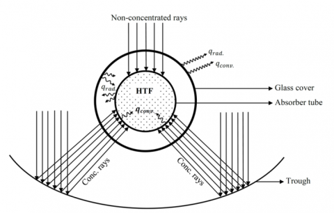
The receiver of a Parabolic Trough Solar Collector (PTSC) is a critical component and the single most expensive equipment in a PTSC power plant [1]. Thus, the primary focus of researchers has been to study the effect of various parameters affecting the receiver of PTSCs, in order to minimize the heat loss from the receiver and improve the PTSC power plant efficiency. Technological improvements like selective coating have been applied on the outer surface of the absorber tube to enhance the absorption of solar rays while reducing the radiation heat loss from that surface. Along with the selective coating, the annulus region between the absorber tube and glass cover in a receiver is evacuated to minimize the convective heat losses from the absorber tube surface (Figure 1).
Several researchers [1-13] have undertaken experimental, analytical and numerical studies on the performance of receiver of PTSC under various working conditions. Experimental investigation of the heat loss from Schott® PTR70 2008 model receiver were carried out by Burkholder and Kutscher [2] with the temperature of receiver ranging from 100-500 °C. Since the absorber tubes have selective coating on their surface, temperature dependent surface emissivity of the absorber tube is a key result from the study. An explicit analytical expression for temperature distribution of an absorber tube of a PTSC system has been provided by Khanna et al. [3]. Optical errors and Gaussian sun shape were considered in their analytical model. Cheng et al. [4] used numerical methods to study the non-uniformity of the solar flux distribution on the absorber tube surface and heat transfer characteristics in PTSC receiver tubes. The numerical analysis was done by combining Monte Carlo Ray-Trace (MCRT) method with Fluent® software. A more detailed analysis using the above technique was presented by He et al. [5]. Wu et al. [6] combined MCRT method with Fluent® for their analysis of parabolic trough receiver and included temperature dependent properties of the heat transfer fluid, the wavelength-dependent optical properties of the receiver surfaces and the glass envelope’s absorption of the solar radiation energy. Parametric numerical investigation of PTSC absorber tubes was carried out by Sahoo et al. [7]. Wind speed, mass flow rate of fluid and incident solar flux were varied and their effect on the absorber tube was studied. The material of the absorber tube was also varied as well to study the circumferential temperature homogeneity. Sivaram et al. [8] presented an experimental and numerical investigation of a PTSC system integrated with a Phase Changing Material (PCM) thermal energy storage system. An experiment was carried out to study the effect of mass flow rate on thermal efficiency. Hachicha et al. [9] developed an optical model for non-uniform flux distribution around the receiver. The results of the optical model were fed into a Finite Volume Method (FVM) model as boundary conditions for further heat transfer calculations. Tripathy et al. [10] have found out the maximum deflection of the PTSC absorber tube for different mass flow rate of the HTF. The materials of the absorber tube were varied to quantify the effect of material on the deflection. Laminated composites as absorber tube material were found to be superior to mono-metallic absorber tubes in minimizing deflection. Habib et al. [11] have used a two band model to divide the solar spectrum for modeling the selective surface of flow receivers of PTSC. An iterative approach is followed for flow calculation of full length absorber tube where in a short section of the receiver is considered for calculation; the outlet values of that section after convergence are fed into the section as inlet condition in the next iteration to simulate the long receiver. Cucumo et al. [12] presents a new model for thermodynamic analysis of PTSC plants. PTSC collector is cooled by air evolving from Joule-Brayton cycle as mentioned in their work. Air as the working substance is inter-cooled in the compressor and regeneration is also used. Year round performance of such plant has also been presented. Odeh and Morrison [13] have presented a simulation model towards optimization of the Parabolic Trough Solar Collector (PTSC) system with storage tank for industrial process heat (IPH) application. To account for unsteady state of solar radiation, transient analysis was adopted. To keep the receiver cost low, a non-evacuated collector was used in their study.
Figure 1. Schematic of the Parabolic Trough Collector System (PTSC) receiver section, showing the non-uniform flux over the receiver circumference
From the literature surveyed, it was inferred that the circumferential temperature difference (∆Tc) and the self-weight of absorber tube are the two biggest factor causing deflection of the absorber tube of a PTSC receiver [10]. The Mass flow rate and the Direct Normal Irradiation (DNI) are the two major factors contributing towards circumferential temperature difference (∆Tc) in the absorber tube. Ray tracing algorithms (MCRT) combined with FVM or FEM is preferred method of numerical solution procedure for performance calculation of PTSC receiver with non-uniform solar loads [4-6]. Most of the simulation procedures have assumed glass cover to be opaque to incoming and outgoing radiation. The solar flux was invariably applied on the inner surface of the absorber tube. Two other factors affecting the performance of PTSC receivers are the inlet temperature of HTF and the wind velocity flowing over the glass cover. Studies highlighting the importance of the two factors on the circumferential temperature difference (∆Tc) of steel absorber tube and glass cover have not been done earlier, as per authors’ knowledge. Therefore parametric studies involving these two parameters have been under taken in this work. The PTSC receiver which has been numerically modeled is having the following features.
Solar flux is applied on the glass cover.
The rest of the paper is structured as follows. The three dimensional computational model developed and the grid generation is covered in section 2. Section 3 covers the mathematical modelling and simulation procedure, which includes the governing equations, numerical methodology, boundary conditions, assumptions, grid independence test and verification of the methodology presented in this paper. The numerical results and detailed discussion on the results are presented in section 4. Section 5 provides a summary of the important findings of this paper.
2.1 Physical setup
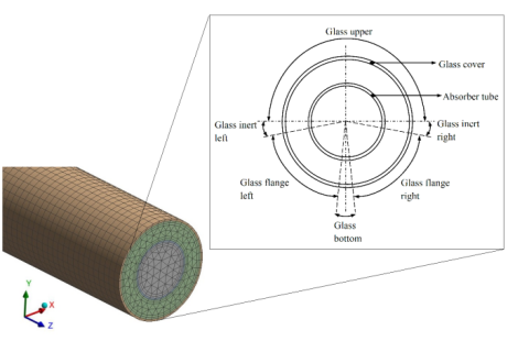
In the current work, the dimensions of PTSC receiver is kept similar to the Schott® PTR70 2008 model receiver. The glass cover of the receiver has an outer diameter of 0.12 m and an inner diameter of 0.115 m. The absorber tube has an outer diameter of 0.070 m and inner diameter 0.066 m [2]. Length of the receiver is taken to be 3.93 m. As the flux is directly applied on the glass cover, to model the circumferential non-uniformity, the glass cover’s outer surface is divided into six divisions. Sector width of the surface divisions are presented in Table 1. For simplification of the model, bellows which are used to attach the glass cover to trough structure and compensate for thermal expansion of absorber tube has not been modeled. The schematic of the surface divisions is presented in Figure 2. For flow to develop, an extra length of 2 m (L/d<25) is provided ahead of inlet of the absorber tube.
Table 1. Width and nature of flux received on the glass cover surface divisions
|
Name |
Sectoral Width (Width in Degrees) |
Nature of Flux Received |
|
Glass Upper |
180° |
Non-concentrated |
|
Glass Bottom |
4° |
No flux received (Shadow region) |
|
Glass Flange Left |
78° |
Concentrated flux |
|
Glass Flange Right |
78° |
Concentrated FLUX |
|
Glass Inert Left |
10° |
No flux received |
|
Glass Inert Right |
10° |
No flux received |
2.2 Grid generation
Hybrid meshing scheme has been adopted for meshing the computational domain. Tetrahedral elements have been used for meshing fluid domains (HTF flow domain and annulus region) and for solid bodies (absorber tube and glass cover) automatic meshing has been adopted. To capture the surface heat transfer phenomena, an inflation layer of hexahedral elements has been provided on the fluid domain surfaces that are in contact with solid surfaces. Figure 2 shows the mesh generated. As the grid independence is checked by refining the grid (Section 3.5) with respect to the rise in the HTF temperature from inlet to outlet of the absorber tube, grid is particularly made finer for fluid domain in the longitudinal direction. Verification of the current methodology entails that grid be finer in the circumferential direction also. Thus, with progression in grid refinement, both longitudinal and circumferential refinement in the grid was carried out till the rise in the HTF temperature (∆Tf=Tout-Tin) did not show appreciable change with further refinement of the grid.
Figure 2. Schematic of the surface divisions and mesh generated
3.1 Governing equations
Since the HTF flow inside the pipe is turbulent (mass flow 8.1 kg/s and 8.8 kg/s), the governing equations [14] for steady flow with conservation of mass, momentum and energy can be written as
Continuity equation
$\frac{∂}{∂x}_i ({pu}_i )=0$ (1)
Momentum equation
$\frac{∂}{∂x_j} (ρu_i u_j )=- \frac{∂p}{∂x_i}+\frac{∂}{∂x_j}[(μ_t+μ)(\frac{∂u_i}{∂x_j}+\frac{∂u_j}{∂x_j})-\frac{2}{3}(μ_t+μ)\frac{∂u_l}{∂x_l}δ_{ij}]+ρg_i$ (2)
Energy equation
$\frac{\partial }{\partial {{x}_{i}}}(\rho {{u}_{i}}T)=\frac{\partial }{\partial {{x}_{i}}}[(\frac{\mu }{\Pr }+\frac{{{\mu }_{t}}}{{{\sigma }_{t}}})\frac{\partial T}{\partial {{x}_{i}}}]+{{S}_{R}}$ (3)
Transport equation for the Standard k-ε model
k equation
$\frac{\partial }{\partial {{x}_{i}}}(\rho {{u}_{i}}k)=\frac{\partial }{\partial {{x}_{i}}}[(\mu +\frac{{{\mu }_{t}}}{{{\sigma }_{k}}})\frac{\partial T}{\partial {{x}_{i}}}]+{{G}_{k}}-\rho \varepsilon $ (4)
ε equation
$\frac{\partial }{\partial {{x}_{i}}}(\rho {{u}_{i}}\varepsilon )=\frac{\partial }{\partial {{x}_{i}}}[(\mu +\frac{{{\mu }_{t}}}{{{\sigma }_{\varepsilon }}})\frac{\partial k}{\partial {{x}_{i}}}]+\frac{\varepsilon }{k}-({{c}_{1}}{{G}_{k}}-{{c}_{2}}\rho \varepsilon )$ (5)
Modelling the turbulent viscosity ( (μ_t )
${{\mu }_{i}}=\rho {{C}_{\mu }}\frac{{{k}^{2}}}{\varepsilon }$ (6)
${{G}_{k}}\text{=}{{\mu }_{t}}\frac{\partial {{\mu }_{i}}}{\partial {{x}_{j}}}(\frac{\partial {{\mu }_{i}}}{\partial {{x}_{j}}}+\frac{\partial {{\mu }_{j}}}{\partial {{x}_{i}}})$ (7)
The model constraints c_1,c_2,C_μ,σ_k,σ_ε,σ_t have the following default values.
${{c}_{1}}=1.44,{{c}_{2}}=1.92,{{c}_{\mu }}=0.09,{{\sigma }_{k}}=1.0,{{\sigma }_{\varepsilon }}=1.3,{{\sigma }_{t}}=0.85.$
G_k represents the generation of turbulence kinetic energy due to the mean velocity gradients.
Turbulent intensity
ki=0.16(Re)-1/8×100% [15] (8)
Heat transfer coefficient
$h=4\times D_g^{-0.42}\times v_w^{0.5}$ [16] (9)
The DO model equation [14, 17].
The radiative transfer equation (RTE) for an absorbing, emitting, and scattering medium is
$\nabla \bullet (I(\overrightarrow{r},\overrightarrow{s})\overrightarrow{s})+(a+{{\sigma }_{s}})I(\overrightarrow{r},\overrightarrow{s})=a{{n}^{2}}\frac{\sigma {{T}^{4}}}{\pi }+\frac{{{\sigma }_{s}}}{4\pi }\int\limits_{0}^{4\pi }{I(\overrightarrow{r},\overrightarrow{s}')}d\Omega '$ (10)
The RTE for the spectral intensity I_λ (r ⃗,s ⃗ ) can be written as
$\nabla \bullet ({{I}_{\lambda }}(\vec{r},\vec{s})\vec{s})+({{a}_{\lambda }}+{{\sigma }_{s}}){{I}_{\lambda }}(\vec{r},\vec{s})={{a}_{\lambda }}{{I}_{b\lambda }}\frac{{{\sigma }_{s}}}{4\pi }\int\limits_{0}^{4\pi }{{{I}_{\lambda }}(\vec{r},{\vec{s}}')}\phi (\vec{s},{\vec{s}}')d{\Omega }'$ (11)
Emissions from wall surface =${{n}^{2}}{{\in }_{w}}\sigma T_{w}^{4}$ (12)
Diffusely reflected energy =${{f}_{d}}(1-{{\in }_{w}}){{q}_{in}}$ (13)
Specularly reflected energy=${{f}_{d}}(1-{{\in }_{w}}){{q}_{in}}$ (14)
Absorption at the wall surface =${{\in }_{w}}{{q}_{in}}$ (15)
Conductivity of the absorber tube
${{k}_{abs}}=14.8+0.0153{{T}_{abs}}$ [18] (16)
3.2 Numerical methodology
The numerical methodology to include the features like selective coating, modeling glass cover as semitransparent and incorporating vacuum in the CFD model are discussed in this section.
Selective coating provided on the outer surface of the absorber tube enhances the absorption of solar insolation while reducing the surface radiation emission. Emissivity (∈) value of a selective coated surface is dependent on surface temperature [2]. The absorptivity (α) of the surface is kept independent (α=0.95) of surface temperature in this work. To model the selective coating, the solar thermal spectrum has been divided into two non-overlapping bands [11]. First band is of 0.1-3 µm and the second is of 3-100 µm. 98 % of the solar radiation is concentrated in the first band [11], while the absorber tube which is comparatively at a very low temperature than the solar surface, emits predominantly in longer wavelengths. Thus, effectively making the first band the absorption band and the second the emission band. The glass cover is modeled semitransparent and flux is applied on the glass outer surface, keeping the directional non-uniformity of the solar flux on the glass surface intact. Glass has different absorption coefficients for different wavelength bands (greenhouse effect); therefore, a non-grey, wavelength banded model for absorption coefficients is used. Vacuum in the annulus region is modeled by making the annulus volume a fluid zone. Convection in the fluid zone (annulus space) is suppressed by using fixed term [19] in the energy equation. In the annulus space cell zone, the x, y, z velocities, turbulent kinetic energy and turbulent dissipation rate are assigned a fixed value [19] of zero. The temperature is kept fixed at 300 K in the annular space.
3.3 Boundary conditions and solver inputs
Suitable boundary conditions are used prior to solving the governing equations. No slip condition has been used at the absorber tube walls. For the HTF flowing inside the absorber tube, mass flow inlet boundary condition has been specified. Turbulent intensity has been arrived at using Eq. (8) after calculation of Reynold’s number. Pressure outlet boundary condition with zero gauge pressure has been used at the outlet of absorber tube. The HTF properties (Table 2) have been defined at the inlet. Sidewalls of the absorber tube, the glass cover and the annular zone have been made adiabatic and do not absorb and emit radiation (a= 0). As discussed in section 3.2, the emissivity (∈) values and the absorptivity (a) values for the selective coating (at absorber outer wall) have been provided. Steel properties used are mentioned in Table 3. Glass properties (Table 3) have been taken constant and are invariant with temperature. Heat flux boundary condition is used for the solar flux which is incident on the glass surface. The value of Direct Normal Irradiation (DNI) used for calculation is 950 W/m2. Value of the concentrated heat flux on the glass surface is arrived at using the geometrical concentration ratio. The nature of flux received by the glass surface divisions are presented in Table 1. Within each surface division constant heat flux is applied. Radiation and convection from the glass cover to the ambient is modeled using mixed boundary condition. The effective heat transfer coefficient (h) for different wind velocities has been calculated from Eq. (9) and applied on the glass surface. Ambient temperature is 300 K. Sky radiation temperature is taken as 295 K.
Steady state pressure based solver is used for the simulations. For turbulence modeling k-ε model with standard wall functions have been used. Discrete Ordinates (DO) model is used for solving the RTE equation. SIMPLEC algorithm has been employed for pressure velocity coupling. Momentum, turbulent kinetic energy, turbulent dissipation rate, energy and discreet ordinates have been discretized with second order upwind scheme, while pressure has been discretized with body force weighted scheme. The convergence criteria for residuals of continuity, x, y, z-velocity, k, ε, DO intensity equations has been kept at 10-4 while for energy equation is the same is 10-6.
Table 2. Table of HTF properties used [20]
|
Sl. No. |
Temperature (K) |
Density (kg/m3) |
Thermal Conductivity (W/m-K) |
Specific Heat (KJ/kg-K) |
Viscosity (mPa-s) |
|
1 |
363 |
1007 |
0.129 |
1.747 |
1.119 |
|
2 |
413 |
965 |
0.123 |
1.886 |
0.642 |
|
3 |
463 |
922 |
0.115 |
2.021 |
0.424 |
|
4 |
513 |
877 |
0.107 |
2.154 |
0.305 |
|
5 |
566 |
828 |
0.098 |
2.287 |
0.232 |
|
6 |
613 |
773 |
0.089 |
2.425 |
0.185 |
|
7 |
663 |
709 |
0.078 |
2.588 |
0.152 |
Table 3. Table of material properties of steel and glass used
|
Material |
Density (kg/m3) |
Thermal Conductivity (W/m-K) |
Specific Heat Capacity (KJ/kgK) |
Refractive index |
|
|
Steel |
8030 |
f(t) (Eq. (16)) |
0.502 |
- |
|
|
Glass [15] |
2225 |
1.1 [2] |
0.835 |
1.1 |
|
3.5 Grid independence test
A grid independence test has been conducted to check the mesh value where the result ceases to be dependent on the grid. Number of elements in the grid has been progressively increased from 103,000 to 612,300 elements. The temperature rises of the HTF from inlet to outlet (∆Tf = Tout-Tin) has been calculated for each grid size investigated, keeping all other parameters constant [10]. A grid with 501,000 elements is chosen for further study since change in ∆Tf presents a change of 0.504% from the previous grid with 425,000 elements and 0.655% to the next higher grid with 612,000 elements. The change observed in ∆Tf is 9.782% when grid size is increased from 103,000 to 425,000. The finding of grid independence test is presented in Figure 3.
Figure 3. Grid independence test
3.6 Verification
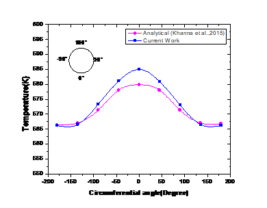
Verification of the current methodology has been done with Khanna et al. (2015) [3]. They [3] have presented an explicit expression for circumferential temperature distribution of the absorber tube. The error observed in the Tp (Peak Temperature) value occurring at the steel bottom (θ=0°), in the current work is 0.08% [10]. The error in the circumferential temperature difference (∆Tc) is 5.27 K from the analytical results [3] and the error can be attributed to the fact that the Gaussian distribution of solar rays over the glass cover surface surface has not been considered in the current work, while [3] have included Gaussian distribution of solar rays (over absorber tube surface) in their results. Figure. 4 represents the comparative graph of circumferential temperature distribution, between current work and explicit expression presented by [3].
Figure 4. Verification of circumferential temperature distribution
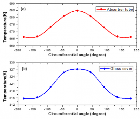
Parametric studies have been conducted by varying the HTF inlet temperature and the wind velocity over the receiver glass cover to study their individual effect on the receiver performance. The circumferential distribution of temperature for the PTSC absorber tube and the glass cover at mid-length is presented in Figure 5 (a) and (b) respectively. The temperature distribution is obtained for a DNI of 950 W/m2, having HTF mass flow rate ($\dot{m}$) of 8.8 kg/s, wind induced heat transfer co-efficient (h) of 13.8 W/m2K and an inlet temperature of 566 K. From Figure 5 (a) and (b) it is seen that the temperature of the outer surface of the absorber tube and the glass cover varies considerably in the circumferential direction. The highest temperature observed is at the bottom position (θ=0°) for both the absorber tube and the glass cover. The lowest temperature is observed at the top position (θ=180°). Both the absorber tube and the glass cover temperature distribution are approximately symmetrical across vertical diametric plane. From Figure 5(a) and (b) it may seem that the absorber tube and the glass cover follow a similar temperature distribution pattern, with the highest and the lowest temperature occurring at similar position, with the exception being the absolute value of the temperatures. But the circumferential temperature difference (∆Tc) also differs. For the absorber tube ∆Tc is 18.72 K whereas for the glass cover ∆Tc is 12.49 K. The circumferential temperature distribution of the glass cover depends upon the temperature distribution of the outer surface of absorber tube, which in turn depends upon the inlet temperature (Tin) of HTF. Other factors that affect the glass cover temperature distribution are DNI (glass cover being semi-transparent), ambient temperature and wind induced heat transfer coefficient (h). Factors like DNI and mass flow rate of HTF, which affect the absorber tube temperature distribution have been widely investigated. Inlet temperature of the HTF and wind induced heat transfer coefficient (h) are two vital factors which affects the absorber tube and glass cover temperature distribution. Thus they have a bearing on the receiver performance and are needed to be investigated. Figure 6 (a), (b) represents the temperature contours of the absorber tube and the glass cover.
Figure 5. Circumferential temperature distribution of (a) absorber tube (b) glass cover at mid-length section, $\dot{m}$ =8.8 kg/s, h=13.8 W/m2K, T=566 K, DNI=950W/m2
Figure 6. Temperature contours of (a) glass cover (b) absorber tube due to non-uniform incident flux over their circumference. $\dot{m}$ =8.8 kg/s, h=13.8 W/m2K, T=566 K, DNI=950W/m2
4.1 Effect of inlet temperature (Tin) variation
Wide range of Tin variations is observed during PTSC plant startup. Apart from startup condition, Tin is dependent on the return loop temperature, which is dependent on the requirement for providing IPH or producing power. In PTSC power plant the return loop temperature depends upon the power cycle (Rankine cycle or Organic Rankine cycle) and design considerations. Thus to encompass all the above factors a large variation of Tin has been studied. Since working limit of Therminol VP1 is 673K [2], the Tin is kept limited to 663 K.
4.1.1 Effect of Tin on circumferential temperature distribution of absorber tube and glass cover
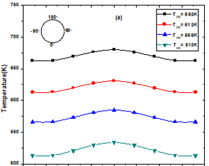
The HTF temperature at the inlet (Tin) has a considerable effect on the circumferential temperature variation. As it can be seen from Figure. 7(a)-(b), average absorber tube temperature (Tav) increases with the increase in the Tin. The peak temperature changes by 72.53 % when Tin changes from 363 K to 663 K. The results are obtained for 950 W/m2 DNI and 8.8 kg/s mass flow rate of the HTF. The circumferential temperature difference (∆Tc) decreases with increase in the Tin. The value of ∆Tc at mid-length section is 30.49 K for 363 K and reduces to 17.08 K when the Tin increases to 663 K. The values of ∆Tc for inlet, mid-length and outlet section of absorber tube for different Tin is presented in Figure. 9. The higher temperature at the inlet can be achieved by either installing auxiliary heating system for HTF in the return loop or through regenerative heating where the HTF at the outlet is bled to heat the HTF in the return loop. A PTSC configuration with regenerative heating or auxiliary heater can be investigated in future.
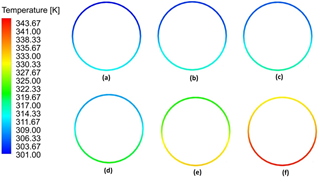
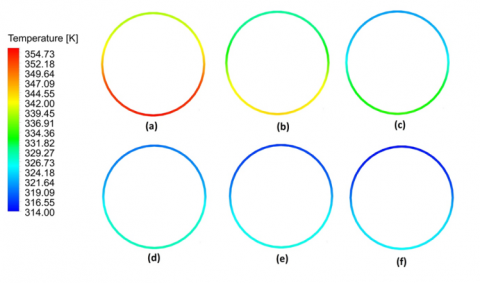
Figure 7(c) represents the circumferential temperature distribution on the glass cover outer surface for different temperature of HTF at inlet. The temperature distribution is obtained by keeping the ambient temperature constant at 300 K and wind induced heat transfer coefficient (h) of 13.8 W/m2 K. The temperature of the glass cover rises as the Tin of the HTF increases. This is due to the fact that the heat radiated from the absorber tube to the glass cover increases as the absorber tube temperature increases with the increase in the Tin. As the radiative heat transferred is related to the fourth power of temperatures of the absorber tube and the glass cover, the peak temperature (θ=0°) of glass cover rises non-linearly, even though the input Tin rise is linear. The peak temperature obtained for Tin 363 K is 313.60 K, which rises to 317.21 K for a Tin of 463 K. Further the peak temperature rises to 344.08 K for Tin of 663 K. The corresponding values of the ∆Tc are 11.92 K, 12.09 K, 12.79 K respectively. For the same values of Tin, absorber tube had larger value of ∆Tc. Thus, for the absorber tube with increase in the Tin, the ∆Tc decreases, while for the glass cover it increases with the increase in the inlet temperature (Tin) of the HTF. The contours for the circumferential temperature distribution in glass cover changes in the Tin are presented in Figure 8.
Figure 7. Circumferential temperature distribution on (a), (b) absorber tube outer surface, (c) glass cover outer surface, for varying temperature of HTF at inlet (Tin). At z=L/2, $\dot{m}$ =8.8 kg/s, h=13.8 W/m2K, DNI=950 W/m2 for steel absorber tube
Figure 8. Temperature contours of glass cover at z=L/2. For $\dot{m}$ =8.8 kg/s, h=13.8 W/m2K, DNI=950 W/m2. (a) 363 K (b) 413 K (c) 463 K (d) 513 K (e) 613 K (f) 663 K
4.1.2 Effect of Tin on temperature rise (∆Tf) and pressure drop of HTF along the length of the absorber tube
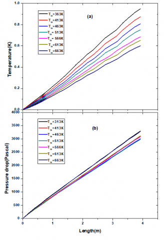
With the increase in the inlet temperature (Tin) of the HTF, axial temperature rise (∆Tf) of the HTF decreases. The values of (∆Tf) are 0.95 K, 0.87 K, 0.80 K, 0.75 K, 0.69 K, 0.65 K, 0.60 K for Tin temperature of 363 K, 413 K, 463 K, 513 K, 613 K and 663 K respectively. The temperature rise of the HTF along the length of the absorber tube for different Tin is represented in the Figure 10 (a). As the ∆Tf value decreases with the Tin, the heat transfer to the HTF also decreases, since the input heat flux is kept constant. This decrease in the ∆Tf value is due to the fact that the temperature gradient between the absorber tube and the HTF mean temperature decreases. In addition to above, the specific heat (cp) and the density (ρ) changes due to change in the HTF temperature, specific heat of Therminol® Vp1 increases with the temperature, but the density decreases [Table 2]. The thermal efficiency of the receiver decreases by 6.45 % when the inlet temperature (Tin) is increased from 363 K to 663 K. Therefore even if a higher operating temperature of the HTF reduces the ∆Tc, the increase in the HTF temperature decreases the heat transferred to the fluid. Therefore, a trade-off becomes necessary between the two factors.
Figure 9. Circumferential temperature difference (∆Tc) on an absorber tube outer surface, with varying temperature of HTF at inlet (Tin). For =8.8 kg/s, h=13.8 W/m2K, DNI=950 W/m2 for steel absorber tube
Density (ρ) of the HTF being a temperature dependent property decreases with the rise in inlet temperature of the HTF [Table 2]. So even though the mass flow at the inlet is constant for all the Tin cases investigated, the volume flow rate does not remain constant. Viscosity of the HTF too changes with the temperature [Table 2]. Therefore the changes in the pressure drop as seen in Figure. 10(b) is due to changes in the fluid properties which are dependent on temperature of the HTF (Tin).
4.2 Effect of convective heat transfer coefficient (h) or effect of wind velocity
4.2.1 Effect of ‘h’ variation on the circumferential temperature distribution of the absorber tube and the glass cover
Glass cover insulates the absorber surface from the wind driven convective heat losses. Thus effectiveness of the glass cover can be tested by varying the wind velocity and measuring the temperature distribution of the absorber tube for changes. As seen from Figure 11(a), the circumferential temperature distribution of the steel absorber tube does not vary significantly with the change in the heat transfer coefficient and the circumferential temperature difference (∆Tc) remains constant at 18.52 K.
Figure 10. Temperature rise of HTF (∆Tf) (a), pressure of HTF along the length of the absorber tube (b), with varying with varying temperature of HTF at inlet (Tin). For $\dot{m}$ = 8.8 kg/s, h = 13.8 W/m2K, DNI = 950 W/m2 for steel absorber tube
The results obtained are for DNI 950 W/m2, mass flow rate of 8.1 kg/s and inlet temperature (Tin) of 613 K. As the wind velocity over the glass cover increases, there is an increase in the heat transfer coefficient (h). This leads to decrease in the glass cover temperature (Figure 11 (b)), thus the radiative heat losses from the absorber tube must increase. The quantum of increase in the radiative heat loss is very small due to the fact that the emissivity of the selective coating is very low (0.086) [2]. Odeh and Morrison [13] had reported a decrease in the overall thermal efficiency at 2.5% for an evacuated receiver. As in the present work, only 3.93 m segment of the receiver is investigated and the selective coating has a very low value of emissivity. Thus, the decrease in the thermal efficiency obtained is very less. But for a non-selectively coated absorber tube the decrease in performance can be considerably higher. Thus the effectiveness of the glass cover in insulating the absorber tube from the environmental factors like wind is established in this work.
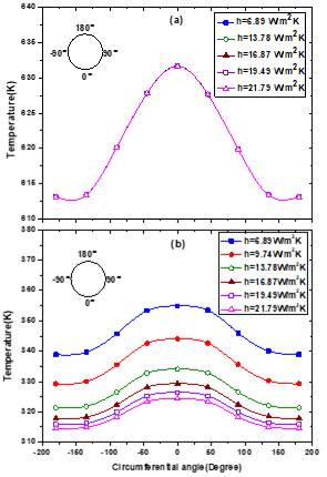
Figure 11. Circumferential temperature distribution on (a) absorber tube outer surface, (b) glass cover for varying heat transfer coefficients (wind velocity). At z = L/2, $\dot{m}$ = 8.1 kg/s, Tin= 613 K, DNI = 950 W/m2 for steel absorber tube
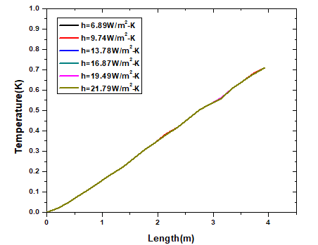
The heat transfer coefficients (h) are calculated from the wind velocities using the Eq. (9). The heat transfer coefficients (h) 6.89 W/m2K, 9.74 W/m2K, 13.78 W/m2K, 16.87 W/m2K, 19.49 W/m2K and 21.79 W/m2K represents a wind velocity of 0.5 m/s, 1 m/s, 2 m/s, 4 m/s and 5 m/s respectively. The direction of the wind flowing over the glass cover is perpendicular to the longitudinal axis of the receiver [16]. As can be seen from Figure 11 (b), the peak temperature (Tp) of the glass cover as well as the circumferential temperature differences (∆Tc) both decreases owing to the increase in the heat transfer coefficient. The decrease in the circumferential temperature difference (∆Tc) or flattening of the curve with rise in the heat transfer coefficient (h) is due to the fact that, heat transfer gets enhanced where the temperature gradient is higher, at the glass bottom (θ=0°). As the correlation between the heat transfer coefficient and the wind velocity is not linear, the rate of rise in the value of the heat transfer coefficient (h) due to increase in the wind velocity, decreases as the wind velocity increases. This coupled with the fact that the temperature gradient between the glass cover surface and the ambient decreases with the increase in wind velocity, the decrease in the peak temperature (Tp) and the average temperature (Tav) of the glass cover is not linear with increase in the wind velocity.
The peak temperature of the glass cover is 354.92 K for a wind velocity of 0.5 m/s and decreases to 324.41 K for a wind velocity of 5 m/s. The change observed is 2.91% when the wind velocity changes from 1 m/s to 2 m/s but the change observed is 0.61% when the wind velocity changes from 4 m/s to 5 m/s. The circumferential temperature difference (∆Tc) decreases from 16.03 K to 9.86 K when the wind velocity increases from 0.5 m/s to 5 m/s. Figure. 12 represents the temperature contours of the glass cover for different heat transfer coefficients (h).
4.2.2 Effect of ‘h’ variation on temperature rise (∆Tf) and pressure drop of HTF along the length of the absorber tube
Since the temperature distribution of the absorber tube approximately remains unaffected due to the change in the heat transfer coefficient (h) (Figure. 11(a)) and the Tin and the mass flow rate ( $\dot{m}$ ) has been kept constant. Therefore the HTF temperature rise along the length of the absorber tube too remains approximately constant as can be seen from Figure. 13. The heat transfer to the fluid also will not change appreciably. Pressure drop along the length of the absorber tube do not show appreciable change for a single PTR 70 (3.93 m) receiver, when the wind velocity increases.But in actual practice where several receivers are linked end to end and installed in loops, some change in pumping power may be observed.
Figure 12. Temperature contours of glass cover at z=L/2. For $\dot{m}$ =8.1 kg/s, Tin=613 K, DNI=950 W/m2. (a) 6.89 W/m2K (b) 9.74 W/m2K (c) 13.78 W/m2K (d) 16.87 W/m2K (e) 19.49 W/m2K (f) 21.79 W/m2K
Figure 13. Temperature of HTF along the length of the absorber tube, with varying heat transfer coefficients (wind velocity). For $\dot{m}$ =8.1 kg/s, Tin=613 K, DNI=950 W/m2 for steel absorber tube
Three dimensional computational model of a PTSC receiver tube was developed and analyzed. Parametric studies were conducted by varying the inlet temperature of HTF (Tin) and varying the wind velocity over the glass cover. The inlet temperature of HTF (Tin) value has been varied from 363 K to 663 K. It was found that the Tin has a considerable effect on the circumferential temperature difference (∆Tc) values.
With increase in the Tin values, the ∆Tc values get reduced but along with it thermal efficiency of the receiver also reduces by 6.45%. Thus a trade-off between the two is required. With increase in the Tin values, the glass cover temperature increases. HTF properties being temperature dependent, slight changes in the pressure drop values are observed. The effectiveness of the glass cover in suppressing the convective heat losses from the absorber tube surface is established in this work. Even though the wind velocity (convective heat transfer coefficient ‘h’) is varied from 0.5-5 m/s, no appreciable change in the circumferential temperature distribution was observed. The glass cover temperature reduces with the increase in ‘h’ values, as more heat is lost from the glass cover surface to the ambient due to convection; the peak temperature (Tp) of the glass cover reduces from 354.92 K to 324.41 K when the wind velocity changes from 0.5 m/s to 5 m/s. Thus, apart from widely investigated parameters like the mass flow rate of HTF and the change in DNI, the inlet temperature of HTF and the wind velocity also have a considerable effect on the performance of the PTSC receiver tube. Parameters such as the inlet temperature of the HTF and local prevailing wind conditions should be studied in conjugation with other parameters, for accurate prediction of the PTSC receiver performance.
Current work can be extended by including other parameters such as variations in the absorber tube thickness, the glass cover thickness. Variation in conditions such as ambient temperature, cloud effect and wind direction can be incorporated into the numerical model. Effect of diffused radiation and ground reflected radiation on the receiver performance can also be studied.
|
Symbol |
Explanation |
|
a |
absorption coefficient (m-1) |
|
a2 |
spectral absorption coefficient |
|
Cp |
specific heat capacity at constant pressure (J.Kg-1.K-1) |
|
c1 , c2 , cu |
coefficients in turbulence model |
|
Dh |
hydraulic diameter(mm) |
|
Dg |
glass diameter(mm) |
|
fd |
diffuse fraction |
|
G |
acceleration due to gravity (m.s-2) |
|
Gk |
turbulent kinetic energy generation rate |
|
h |
convective heat transfer coefficient on outer surface of glass cover (W/ K) |
|
I |
radiation intensity, which depends on position ( $\vec{r}$ ) and direction ( $\vec{r}$ ) (W.sr-1) |
|
Ibλ |
black body intensity given by the Planck function (W.sr-1.m-1) |
|
Iλ |
spectral intensity (W.sr-1.m-1) |
|
k |
thermal conductivity of absorber tube (W.m-1.K-1) |
|
L |
length of absorber tube(m) |
|
$\dot{m}$ |
mass flow rate(kg.s-1) |
|
n |
refractive index |
|
q |
heat loss (W) |
|
r |
radius(mm) |
|
$\vec{r}$ |
position vector |
|
Re |
Reynolds number |
|
s |
path length |
|
$\vec{s}$ |
direction vector |
|
$\vec{s}$' |
scattering direction vector |
|
SR |
source term (W.m-3) |
|
T |
temperature(K) |
|
Tav |
average temperature(K) |
|
Tp |
peak temperature(K) |
|
∆Tf |
HTF temperature change per unit length (K.m-1) |
|
∆Tc |
circumferential temperature difference (K) |
|
Tw |
wall temperature(K) |
|
vw |
wind velocity(m.s-1) |
|
Z |
axial distance(mm) |
|
Abbreviation |
Word(s) |
|
DNI |
direct normal irradiance |
|
FVM |
finite volume method |
|
HTF |
heat transfer fluid |
|
IPH |
industrial process heating |
|
PCM |
phase changing materials |
|
PTSC |
parabolic trough solar collector |
|
MCRT |
Monte Carlo ray trace |
|
SIMPLEC |
semi-implicit method for pressure linked equations-consistent |
|
a |
absorptivity of absorber tube |
|
∈ |
emissivity |
|
ρ |
density (kg.m-3) |
|
Θ |
circumferential angle or polar angle |
|
σt |
turbulent Prandtl number |
|
σk |
turbulent Prandtl number for turbulence kinetic energy |
|
σε |
turbulent Prandtl number for turbulent kinetic energy dissipation rate |
|
σs |
scattering coefficient |
|
μt |
turbulent viscosity (kg.m-1.s-1) |
|
σ |
Stefan-Boltzmann constant (W.m-2.K-4) |
|
kin |
turbulent intensity |
|
k |
turbulence kinetic energy (m2.s-2) |
|
ε |
turbulent kinetic energy dissipation rate (m2.s-3) |
|
$\Phi $ |
phase function |
|
λ |
wavelength (m) |
|
Ω |
solid angle (sr) |
|
∈w |
wall emissivity |
|
Abs |
absorber tube |
|
av |
average |
|
c |
circumferential |
|
Conv. |
convection |
|
f |
fluid |
|
I |
Intensity |
|
in |
inlet |
|
out |
outlet |
|
p |
peak |
|
Rad. |
radiation |
|
T |
turbulent |
[1] Hachicha AA. (2013). Numerical modeling of a parabolic trough solar collector. Universitat Politècnica de Catalunya, Barcelona, Spain.
[2] Burkholder F, Kutscher C. (2009). Heat loss testing of Schott’s 2008ptr70 parabolic trough receiver. National Renewable Energy Laboratory, Golden, CO, United States. Technical Report No.NREL/TP-550-45633. https://doi.org/10.2172/1369635
[3] Khanna S, Singh S, Kedare SB. (2015). Explicit expressions for temperature distribution and deflection in absorber tube of solar parabolic trough concentrator. Solar Energy 114: 289-302. https://doi.org/10.1016/j.solener.2015.01.044
[4] Cheng ZD, He YL, Xiao J, Tao YB, Xu RJ. (2010). Three dimensional numerical study of heat transfer characteristics in the receiver tube of parabolic trough solar collector. International Communication in Heat Mass Transfer 37: 782-787. https://doi.org/10.1016/j.icheatmasstransfer.2010.05.002
[5] He YL, Xiao J, Cheng ZD, Tao YB. (2011). A MCRT and FVM coupled simulation method for energy conversion process in parabolic trough solar collector. Renewable Energy 36: 976–985. https://doi.org/10.1016/j.renene.2010.07.017
[6] Wu Z, Li S, Yuan G, Lei D, Wang Z. (2014). Three-dimensional numerical study of heat transfer characteristics of parabolic trough receiver. Applied Energy 113: 902-911. https://doi.org/10.1016/j.apenergy.2013.07.050
[7] Sahoo SS, Singh S, Banerjee R. (2010). Parametric studies on parabolic trough solar collector. World Renewable Energy Congress XI (WREC), Abu Dhabi, UAE, pp. 1775-1781.
[8] Sivaram PM, Nallusamy N, Suresh M. (2016). Experimental and numerical investigation on solar parabolic trough collector integrated with thermal energy storage unit. International Journal of Energy Research 40: 1564-1575. https://doi.org/10.1002/er.3544
[9] Hachicha AA, Rodriguez I, Capdevila R, Oliva A. (2013). Heat transfer analysis and numerical simulation of a parabolic trough solar collector. Applied Energy 111: 581-592. https://doi.org/10.1016/j.apenergy.2013.04.067
[10] Tripathy AK, Ray S, Sahoo SS, Chakrabarty S. (2018). Structural analysis of absorber tube used in parabolic trough solar collector and effect of materials on its bending: A computational study. Solar Energy 163: 471-485. https://doi.org/10.1016/j.solener.2018.02.028
[11] Habib L, Hassan MI, Shatilla Y. (2015). A realistic numerical model of lengthy solar thermal receivers used in parabolic trough CSP plants. The 7th International Conference on Applied Energy – ICAE2015, Energy Procedia 75: 473-478. https://doi.org/10.1016/j.egypro.2015.07.427
[12] Cucumo M, Ferraro V, Kaliakatsos D, Marinelli V. (2013). A calculation model for a thermodynamic analysis of solar plants with parabolic collectors cooled by air evolving in an open joule-Brayton cycle. International Journal of Heat and Technology 31(2): 111-118. https://doi.org/10.18280/ijht.310215
[13] Odeh SD, Morrison GL. (2006). Optimization of parabolic trough solar collector system. International Journal of Energy Research 30: 259-271. https://doi.org/https://doi.org/10.1002/er.1153
[14] Cheng ZD, He YL, Cui FQ, Xu RJ, Tao YB. (2012). Numerical simulation of parabolic trough solar collector with non-uniform solar flux conditions by coupling FVM and MCRT method. Solar Energy 86: 1770-1784. https://doi.org/10.1016/j.solener.2012.02.039
[15] Tijani AS, Roslan AMSB. (2014). Simulation analysis of thermal losses of parabolic trough solar collector in Malaysia using computational fluid dynamics. 2nd International Conference on System-Integrated Intelligence: Challenges for Product and Production Engineering, Procedia Technology 15: 841–848. https://doi.org/10.1016/j.protcy.2014.09.053
[16] Mullick SC, Nanda SK. (1989). An improved technique for computing the heat loss factor of a tubular absorber. Solar Energy 42: 1-7. https://doi.org/10.1016/0038-092X(89)90124-2
[17] ANSYS, Inc. Canonsburg, PA. ANSYS Fluent 16.0 Tutorial Guide, 2016. https://www.scribd.com/document/262824146/ANSYS-Fluent-Tutorial-Guide/, accessed on Jan. 10, 2018.
[18] Forristall R. (2003). Heat transfer analysis and modeling of a parabolic trough solar receiver implemented in engineering equation solver. National Renewable Energy Laboratory, Golden, CO, United States. Technical Report No. NREL/TP-550-34169. https://doi.org/10.2172/15004820
[19] Das K, Basu D. Software Validation Plan and Report for Ansys-Fluent version 12.1, Center for Nuclear Waste Regulatory Analysis, San Antonio, Texas, 7.2.
[20] Therminol VP-1. Vapor Phase/ Liquid Phase Heat Transfer Fluid (Liquid Phase), Solutia Inc, 2017. http://twt.mpei.ac.ru/tthb/hedh/htf-vp1.pdf/, accessed on Mar. 12, 2018.