OPEN ACCESS
Magnetic refrigeration is an ecofriendly solid state technology employing magnetocaloric materials in an Active Magnetic Regenerating refrigerant cycle (AMR), a Brayton-based thermodynamical cycle. Magnetic refrigeration is based on magnetocaloric effect (MCE), a physical phenomenon that couples an external magnetic field with the magnetic moments of magnetocaloric materials. In the case of ferromagnetic materials, MCE is a warming as the magnetic moments of the atom are aligned by the application of a magnetic field, and the corresponding cooling upon removal of the magnetic field. Gadolinium is the benchmark material for magnetic refrigeration in room temperature range, thanks to its marked magnetocaloric effect which is maximum at 294 K. In this paper the results of numerical investigations on magnetocaloric materials are presented: the energetic performances of different magnetocaloric materials have been investigated through a two-dimensional model of an AMR regenerator. The model has been previously experimentally validated with a Rotary Permanent Magnet Magnetic Refrigerator. Exploring the behavior of the regenerator under variable working condition, a performance map has been obtained for gadolinium. The results, collected in terms of temperature span, coefficient of performance and mechanical power associated to circulation pump, lead to formulize viewpoints on employing magnetocaloric materials under optimized AMR working conditions.
magnetic refrigeration, AMR, numerical model, gadolinium, performance map
In a world where nearly 17% of the overall energy consumption originates from refrigeration and where R134a is still the most employed refrigerant for domestic scopes, a substantial conversion to the utilization of environmentally friendly refrigerants has become a “must”. As a matter of fact, most modern refrigeration units are even based on Vapor Compression Plants (VCP) in which the characteristics of the working refrigerant have often carried to critical points. The traditional refrigerant fluids, i.e. CFCs and HCFCs, linked to the beginning of their commercial diffusion, have been banned by the Montreal Protocol [1] because of their significant Ozone Depletion Potential (ODP) [2-4]. Therefore, over time, the focus has been progressively shifted on zero ODP refrigerants but most of the refrigerants nowadays employed, like R134a, shows a relevant direct impact on global warming, who has been quantified through a parameter called GWP (Global Warming Potential). The Kyoto Protocol [5], under the United Nations Framework Convention on Climate Change (UNFCCC), fixed mandatory targets for greenhouse gas emissions, calling the all over the world countries for a phase down of HFC consumption [6, 7].
Human activities have increased the energy consumption in buildings [8-12], because of the growing HVAC employment, environmental pollution [13] and the concentration of greenhouse gases in the atmosphere. This resulted in a substantial heating of the land surface and atmosphere that adversely affected the natural ecosystem. Therefore, nowadays the use of environmentally friendly refrigerants has become a “must” to mitigate the global heating. In this context, scientific community has devoted the attention on other concepts of refrigeration and on no-fluid-state refrigerants.
In the general framework of new refrigerating technologies, solid state coolings are gaining more and more attentions, due to their potential in being performing and ecological methodologies [14]. Recent discoveries of giant caloric effects in some ferroic materials have opened the door to the use of solid-state materials as an alternative to gases for conventional and cryogenic refrigeration. Among them electrocaloric [15, 16] and magnetocaloric cooling [17], seems to be really promising since could constitute a real chance to overcome vapor compression refrigeration limits.
Magnetic refrigeration is an ecofriendly [18] solid state technology employing magnetocaloric materials in an Active Magnetic Regenerating refrigerant cycle (AMR), a Brayton-based thermodynamical cycle. An AMR cycle consists of two adiabatic stages (magnetization–demagnetization) and two isofield stages, corresponding to the heat transfer fluid flowing through the regenerator, whom is the core of a magnetic refrigerator since it plays a dual-role: it operates both as refrigerant and as regenerator in an AMR cycle. Magnetic refrigeration is based on magnetocaloric effect (MCE), a physical phenomenon that couples an external magnetic field with the magnetic moments of magnetocaloric materials, carried by itinerant or localized electrons. In the case of ferromagnetic materials, MCE is a warming as the magnetic moments of the atom are aligned by the application of a magnetic field, and the corresponding cooling upon removal of the magnetic field. Gadolinium is the benchmark material for magnetic refrigeration in room temperature range, thanks to its marked magnetocaloric effect which is maximum at 294 K. The core of a magnetic refrigerator is the regenerator: the best solution is the employment of Active Magnetic Regenerators (AMR), where the magnetic material acts both as refrigerant and as regenerator.
In this paper the energetic performances of an AMR refrigerator have been investigated through the development of a two-dimensional model [19] that can reply the behavior of one of the AMR regenerators employed in “8Mag”, the experimental prototype of the first italian Rotary Permanent Magnet Magnetic Refrigerator (RPMMR) [20].
The MagnetoCaloric Effect (MCE) is a physical phenomenon detected for the first time in iron, in 1881 [21], as temperature change in the material by varying the intensity of the magnetic field applied, under adiabatic conditions. The entropy of a magnetic solid at constant pressure S(T, H) is a function of both the magnetic field intensity H and the absolute temperature T and it consists of three contributions: magnetic (SM), lattice (Slat) and electronic (Sel) ones:
$S=S_{M}(T, H)+S_{l a t}(T)+S_{e l}(T)$ (1)
In equation (1), the magnetic contribution is function of both H and T, whereas the electronic and lattice contributions only depend on T. Consequently, only the magnetic entropy SM can be controlled by varying the magnetic-field strength. When the magnetic field is applied to a magnetic material, the magnetic dipoles become oriented along the direction of the field. If this is done isothermally, it carries to a decrement of the material’s magnetic entropy by the isothermal entropy decreasing (ΔSM)T. The entropy change can be evaluated as:
$\left(\Delta S_{M}\right)_{T}=\int_{H_{i}}^{H_{f}}\left(\frac{\partial M}{\partial T}\right)_{H} d H$ (2)
On the other side, if the magnetization is done adiabatically, the total sample entropy remains constant and the decrease in magnetic entropy is countered by an increase in the lattice and electron entropy. This causes a heating of the material and it takes an increasing of its temperature given by the adiabatic temperature change, ΔTad. Dually, an adiabatic demagnetization involves the increasing of the material's magnetic entropy, causing a decreasing in lattice vibrations and by that a temperature decrease. The expression for ΔTad of a magnetic material can be evaluated as:
$\left(\Delta T_{a d}\right)_{s}=-\int_{H_{i}}^{H_{f}} \frac{T}{C_{H}}\left(\frac{\partial M}{\partial T}\right)_{H} d H$ (3)
where the specific heat can be defined as:
$\mathrm{C}_{\mathrm{H}}=\mathrm{T}\left(\frac{\delta \mathrm{s}}{\delta \mathrm{T}}\right)_{\mathrm{H}}$ (4)
At the Curie temperature, a magnetic material exhibits its maximum MCE. There are two types of magnetic phase changes that may occur at the Curie point: First Order Magnetic Transition (FOMT) and Second Order Magnetic Transition (SOMT). A FOMT material shows a discontinuity in the first derivative of the Gibbs free energy, whereas in a SOMT material the first derivative is a continuous function and discontinuity takes place in the second derivative. Therefore, in a FOMT material the magnetization, i.e. the first derivative of the free energy with respect to the applied magnetic field strength, is discontinuous. In a SOMT material the magnetic susceptibility, i.e. the second derivative of the free energy with the field strength, changes discontinuously. Most of the magnetic materials order with a SOMT from a paramagnet to a ferromagnet, ferrimagnet or antiferromagnet [18]. The benchmark material of magnetic refrigeration is gadolinium (Gd), a rare earth which exhibits a SOMT at TCurie=294 K and it belongs to lanthanide group of elements.
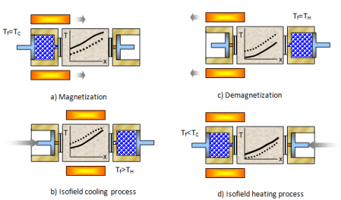
The referring thermodynamical cycle of magnetic refrigeration is the reverse Brayton cycle [22] and, as a matter of fact, in 1982 Barclay introduced an innovative way to follow it up by the introduction of the AMR cycle [23]. The AMR couples into a single concept what had been before two separate processes: instead of using a different material as a regenerator to recuperate heat from the magnetic material, the AMR concept made use of the refrigerant magnetic material itself. A temperature gradient is established throughout the AMR and a fluid is used to transfer heat from the cold to the hot end. The working principle of an AMR is presented in Figure 1 where: the dashed line represents the initial temperature profile of the bed in each process, the solid line depicts the final temperature profile of the process.
Figure 1. The four processes of an AMR cycle related to an AMR regenerator kept in contact with a cold and a hot heat exchanger
If the bed is in steady state condition, with the hot heat exchanger at TH and the cold heat exchanger at TC, four processes constitute the AMR cycle:
(a) Adiabatic magnetization: each particle of the magnetic material which constitutes the regenerator, warms up by increasing progressively the intensity of the magnetic field applied, under adiabatic conditions;
(b) isofield cooling: with the magnetic field at maximum value, the fluid blows from the cold to the hot end of the regenerator. Therefore, the regenerator cools down, transferring heat to the fluid, expelled in the hot heat exchanger;
(c) adiabatic demagnetization: by decreasing adiabatically the intensity of the magnetic field applied from a maximum until a minimum value, the regenerator cools anymore and a decrement of temperature, equal to ∆Tad(T) is registered;
(d) isofield heating: while magnetic field has kept to a minimum value, the fluid flows from the hot to the cold end; thus, the fluid, hotter, cools itself by crossing the regenerator and reaching a temperature lower than TC. At this stage the secondary fluid absorbs heat from the cold heat exchanger at TC, producing a cooling load.
In this paper is introduced a two-dimensional model of a packed-bed AMR regenerator operating at room temperature.
As visible in Figure 2, the regenerator has a rectangular shape with a height of 20mm and a length of 45 mm; the area of the regenerator is filled with a regular matrix of 3600 circles that constitute the solid-state refrigerant; every circle has a diameter of 0.45mm and the amount of the area occupied by all the circles is 63% of the total rectangular area. A group of channels is formed by stacking particles in the regenerator area: the fluid flows through these interstitial channels. The fluid flow in the positive x direction during the isofield cooling process and in the opposite direction during isofield heating.
Figure 2. Packed-bed AMR regenerator
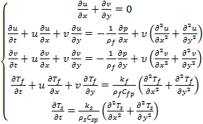
The mathematical formulation that describes the AMR cycle includes several distinct groups of equations with respect to the different processes of the AMR cycle that the regenerator experiences. The equations that rule the regenerative fluid flow processes, in both directions, are: the Navier-Stokes equations for the fluid flow and the energy equations for both the fluid and the solid particles. The fluid is sufficiently low speed to be considered laminar. The solid and the fluid temperature are strictly related and they are constantly evolving during the whole AMR cycle. With the assumptions that the wrapper is adiabatic, the fluid is incompressible, the viscous dissipation is neglected, due to low mass flow, the equations during the fluid flowing phases of the AMR cycle, are:
(5)The equations that model magnetization and demagnetization processes are:
$\left\{\begin{array}{c}{\rho_{\mathrm{f}} \mathrm{C}_{\mathrm{fp}} \frac{\partial \mathrm{T}_{\mathrm{f}}}{\partial \mathrm{t}}=\mathrm{k}_{\mathrm{f}}\left(\frac{\partial^{2} \mathrm{T}_{\mathrm{f}}}{\partial \mathrm{x}^{2}}+\frac{\partial^{2} \mathrm{T}_{\mathrm{f}}}{\partial \mathrm{y}^{2}}\right)} \\ {\rho_{\mathrm{s}} \mathrm{C}_{\mathrm{H}} \frac{\partial \mathrm{T}_{\mathrm{s}}}{\partial \mathrm{t}}=\mathrm{k}_{\mathrm{s}}\left(\frac{\partial^{2} \mathrm{T}_{\mathrm{s}}}{\partial \mathrm{x}^{2}}+\frac{\partial^{2} \mathrm{T}_{\mathrm{s}}}{\partial \mathrm{y}^{2}}\right)+\mathrm{Q}}\end{array}\right.$ (6)
The model considers magnetocaloric effect which elevates or reduces the temperature of the solid by the variation of the external magnetic field applied to the regenerator. Hence the MCE temperature variation ∆Tad is converted [18] into a heat source Q:
$\mathrm{Q}=\mathrm{Q}\left(\mathrm{H}, \mathrm{T}_{\mathrm{S}}\right)=\frac{\rho_{\mathrm{s}} \mathrm{C}_{\mathrm{H}}\left(\mathrm{H}, \mathrm{T}_{\mathrm{s}}\right) \Delta \mathrm{T}_{\mathrm{ad}}\left(\mathrm{H}, \mathrm{T}_{\mathrm{s}}\right)}{\tau}$ (7)
which has the dimensions of a power density and included in the solid energy equation, only for magnetization and demagnetization phases. The term Q is positive during magnetization, negative during demagnetization. τ is the period of the magnetization/demagnetization process. The coupled equations that govern the AMR cycle, imposed on this model, are solved using Finite Element Method.
The AMR cycle is modeled as four sequential steps. The same time step τ has been chosen for the resolution during all the four periods of the cycle. The cycle is repeated several times with constant operating frequency until the regenerator reaches steady state operation.
The model has been developed, as a primary purpose, to be able to reproduce the behavior of one of the regenerator of the RPMMR [20], developed at the University of Salerno. To this aim, the model has been experimentally validated with experimental results provided by the prototype. This model is used to optimize the experimental device and to identify significant areas of device improvement. Thus, it has been used to explore the critical aspects of 8Mag and to outline the way to improve performance. The model has been validated: 1) at zero-load conditions, where no cooling load has been introduced, as a function of AMR cycle frequency; 2) at fixed cooling load, as a function of AMR cycle frequency.
4.1 Zero-load tests
To validate the model, as first step, zero-load tests have been performed. In all simulations, the fluid is pure water and the solid is pure gadolinium [24]. Both the model simulations and the RPMMR tests were performed with a fluid flow rate fixed at 7.0 l*min-1 (normal velocity speed fixed at 0.08335 m*s-1), while the AMR cycle frequency was varied in the range 1.08÷1.79 Hz. The heat rejection temperature, TH, was also varied over the range of 289÷302 K to characterize the performance sensitivity to the heat rejection temperature in the proximity of the refrigerant Curie temperature.
The results collected at zero load tests are presented in terms of ∆TAMR, the zero-load ∆Tspan, evaluated as the difference between the temperature of the hot heat exchanger and the temperature of the regenerating fluid exiting the cold side, at the end of an AMR cycle working in steady-state conditions.
The experimental and model results are plotted in Figure 3 (a), (b), (c), (d). The general trend shows that the zero-load temperature span (∆TAMR) increased with the increasing hot-side temperature, reaching a maximum and decreasing afterward. The maximum for both the experimental and model results corresponded to a hot side temperature of approximately 298 K. Corresponding to this hot side temperature, the average temperature of the bed was near the Curie temperature of gadolinium, where the magnetocaloric effect was at its maximum.
The general trend of the model is to overestimate the experimental data. The overestimating is slight for low hot side temperatures and, overall, for low cycle frequencies. The differences between the experimental and model results increase with increasing cycle frequency. The differences vary between a minimum value of +2% (at 1.25 Hz) and a maximum value of +40% (at 1.79 Hz), with a mean value of approximately +7%.
Figure 3. Comparison between experimental and simulation results in terms of ∆TAMR as a function of TH at fAMR of (a)1.08, (b)1.25, (c)1.61 and (d)1.79 Hz
4.2 Iso-load tests
After validated the model at zero-load, other campaigns of both experimental tests and numerical simulation have been scheduled to estimate the accuracy of the results carried by the developed two-dimensional model with the ones provided by RPMMR, when a fixed cooling power has been applied to the system.
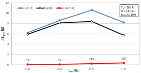
The tests have been performed as a function of fAMR with 296 K as temperature of hot heat exchanger, a fluid flow rate of 5 l/min and a cooling power of 55W.
Figure 4 reports the results collected in terms of temperature span, evaluated as:
$\Delta T_{s p a n}=T_{H}-\int_{t_{M}+t_{C F}+t_{D}}^{t_{M}+t_{C F}+t_{D}+t_{H F}} T_{f}(0, y, t) d t$ (8)
Figure 4 reveals that, with the assumed operative conditions, temperature span increases with the AMR frequency until it reaches a maximum around 0.77 Hz, for both the experimental and numerical results, and decreases afterward. As already detected in the zero-loaf tests, the general trend of the model is to overestimate the experimental results: the difference increases with increasing fAMR and it varies from a minimum value of +5% (0.38 Hz), to a maximum of +33 % (1.25 Hz), with a mean value of +16%. Such difference is given by the presence of Eddy currents during the prototype working, that afflict its performance as much as higher is the operating frequency.
Figure 4. Comparison between experimental and numerical results in terms of ∆Tspan as a function of fAMR
5.1 Numerical simulations
Several AMR cycles have been simulated through the 2D model, under a number of different operative conditions, in order to carry out a map of performances of the AMR regenerator. Frequency of AMR cycle has been varied over a [0.38÷1.25] Hz, together with fluid flow rate [5÷21] l/min and temperature of cold [286÷292] K and hot [295÷302] K heat exchangers. All the tests presented in this section have been conducted employing gadolinium as refrigerant, in order to explore virtually the behavior of the RPMMR under a huge number of different scenarios. Afterwards the performance map has been extended to other solid-state refrigerants for magnetic refrigeration at room temperature.
Measurements of temperature span (defined in equation (8)), coefficient of performance and mechanical power associated to the circulation pump have been performed.
The coefficient of performances has been evaluated as follows:
$C O P=\frac{\dot{Q}_{r e f}}{\dot{Q}_{H}-\dot{Q}_{r e f}+\dot{W}_{p}}$ (9)
where Q'ref is the cooling power, evaluated as follows:
$\dot{Q}_{\text {ref }}=\frac{1}{\theta} \int_{\mathrm{t}_{\mathrm{M}}+\mathrm{t}_{\mathrm{CF}}+\mathrm{t}_{\mathrm{D}}}^{\mathrm{t}_{\mathrm{M}}+\mathrm{t}_{\mathrm{CF}}+\mathrm{t}_{\mathrm{D}}+\mathrm{t}_{\mathrm{HF}}} \dot{\mathrm{m}}_{\mathrm{f}} \mathrm{C}_{\mathrm{f}}\left(\mathrm{T}_{\mathrm{C}}-\mathrm{T}_{\mathrm{f}}(0, \mathrm{y}, \mathrm{t})\right) \mathrm{dt}$ (10)
Q'H is the power related to the heat supplied in the environment which has been evaluated as:
$\dot{\mathrm{Q}}_{\mathrm{H}}=\frac{1}{\theta} \int_{\mathrm{t}_{\mathrm{M}}}^{\mathrm{t}_{M}+\mathrm{t}_{\mathrm{CF}}} \dot{\mathrm{m}}_{\mathrm{f}} \mathrm{C}_{\mathrm{f}}\left(\mathrm{T}_{\mathrm{f}}(\mathrm{L}, \mathrm{y}, \mathrm{t})-\mathrm{T}_{\mathrm{H}}\right) \mathrm{d} \mathrm{t}$ (11)
W’p is the mechanical power associated to the circulation pump:
$\dot{\mathrm{W}}_{\mathrm{p}}=\frac{\mathrm{m}\left(\Delta p_{\mathrm{CF}}+\Delta \mathrm{p}_{\mathrm{HF}}\right)}{\eta_{\mathrm{p}} \rho_{\mathrm{f}}}\left(\mathrm{t}_{\mathrm{CF}}+\mathrm{t}_{\mathrm{HF}}\right)$ (12)
5.2 Results
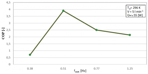
Figure 5. Coefficient of performance as a function of fAMR
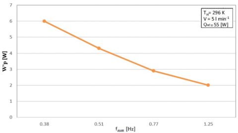
Figure 6. Mechanical power as a function of fAMR
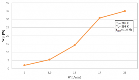
Figure 7. Mechanical power as a function of flow rate
Figure 5 reports COP as a function of AMR frequency, with fixed hot reservoir temperature (296 K), cooling load (55 W) and flow rate (5 l/min). The peak (3.9), in the abovementioned condition, is registered for fAMR = 0.51 Hz, whereas values belonging to [2, 2.5] are found for higher frequencies up to 1.25 Hz; contrariwise, when the regenerator works at frequencies lower than 0.51 Hz, coefficient of performance decay sharply, until reaching a value of 0.7 at fAMR = 0.38 Hz. The reason of such performance falling, must be found in the influence on COP of the mechanical power associated to the circulation pump.
As clearly visible in Figure 6, W’p becomes the more significant the lower is AMR frequency and, therefore, the higher becomes time of fluid flow processes in the AMR cycle. Even if we fix the operating frequency at 1.25 Hz (where W’p is the minimum value registered) while increasing V’, as Figure 7 reveals, the influence of pressure drops becomes so large as to make it impossible to use the packed bed configuration by about 8-10 l/min onwards.
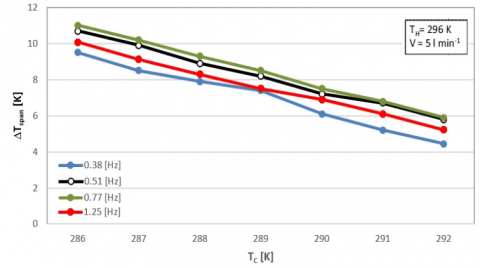
Figure 8. ∆Tspan as a function of cold heat exchanger temperature for a number of fAMR
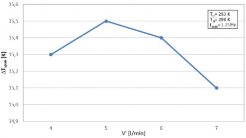
Figure 9. ∆Tspan as a function of fluid flow rate
Figure 10. COP as a function of fluid flow rate
Figure 8 shows the ∆Tspan trend as a function of cold heat exchanger temperature, for a number of AMR frequencies. As predicted by Figure 4, the highest ∆Tspan values have to be attributed at fAMR = 0.77 Hz even if, by increasing TC, they become comparable with ∆Tspan at fAMR = 0.51 Hz. It is important to note that, as it is conceived for equation (8), ∆Tspan is always as greater as wider is the TC÷TH range; what is useful to better appreciate the performance is the temperature gain given by:
$\mathrm{G}_{\mathrm{T}}=\Delta \mathrm{T}_{\mathrm{span}}-\left(\mathrm{T}_{\mathrm{H}}-\mathrm{T}_{\mathrm{C}}\right)$ (13)
As a matter of fact, still referring to Figure 8, the highest performances are given by fAMR = 0.77 Hz in the 288÷296 K range, where GT = 1.5 K; in 286÷296 K range, even if ∆Tspan is the greater (∆Tspan = 11 K, with fAMR = 0.77 Hz) the gain registered is GT = 1 K.
It is interesting to monitor how the AMR regenerator works in limit conditions for its usage: a number of results have been carried out in 283÷298 K range where, therefore the difference between cold and hot heat exchanger amounts to 15 K. Figure 9 and Figure 10 exhibit respectively ∆Tspan and COP as a function of fluid flow rate, in 283÷298 K range, at fAMR = 1.25 Hz. From Figure 9 it is appreciable how GT does not exceed 0.5, since 283÷298 K is a too large range as to enable the regenerator working efficiently. The same is detected in Figure 10, where coefficient of performance does not surpass the value of 0.4.
6.1 Features of the materials
After built a map of performance of the AMR regenerator, working with gadolinium, another investigation has been done through the 2D model, employing other possible refrigerants for magnetic refrigeration at room temperature. Next to gadolinium and considering the criteria [18] to identify a good candidate for magnetic refrigeration, it has been tested a number of different materials, whose MCE is significant at room temperature. Table 1 summarize the characteristics of the materials. The main parameters of the different materials allow a fast comparison in terms of cost vs performance analysis. ΔTad and ΔSM reported are the peak value, at Curie temperature (TCurie) with a magnetic field variation ΔH of 1.5 T.
Table 1. Features of the materials
|
Materials |
TCurie [K] |
∆Tad [K] |
∆SM [J/kg K] |
Cost [€/kg] |
|
Gd |
294 |
6 |
5 |
3000 |
|
Gd5(Si2Ge2) |
276 |
7.8 |
14 |
9000 |
|
LaFe11.384 Mn0.356Si1.26H1.52 |
290 |
5 |
10.5 |
1200 |
|
LaFe11.05Co0.94Si1.10 |
287 |
3.17 |
5.5 |
1200 |
|
MnFeP0.45As0.55 |
307 |
4 |
12 |
1500 |
|
Pr0.65Sr0.35MnO3 |
295 |
1.5 |
2.5 |
1050 |
Table 1 allows a quick comparison between the different magnetic materials. Gd5(Si2Ge2) shows the higher peak values, but out of the room temperature range. The greater thermal conductivity is that of Gd, but also LaFeSi alloys show high values. From a commercial point of view, Gd5(Si2Ge2) and Gd are too expensive and the magnetic transition metals are more adequate than the rare earths for an industrial production of magnetic cooling engines. La is the cheapest element of the rare-earths series, and Fe, Si, Mn are available in large amounts. Cost of MnFeP0.45As0.55 is quite low, but processing of as is complicated due to its toxicity.
6.2 Numerical simulations
Several AMR cycles with different magnetocaloric materials employed as refrigerant, were simulated. The simulations were performed with fixed flow rate (5 l/min) and AMR cycle frequency (1.25 Hz) so that pressure drops do not afflict significantly the performance of the regenerator in terms of COP. The cold heat exchanger temperature TC (288 K). The hot heat exchanger temperature TH was varied in the range 295÷302 K to characterize the performance sensitivity of the heat rejection temperature in proximity of the refrigerant Curie temperature.
6.3 Results
Measurements of temperature span (defined in equation (8)) and coefficient of performance have been performed.
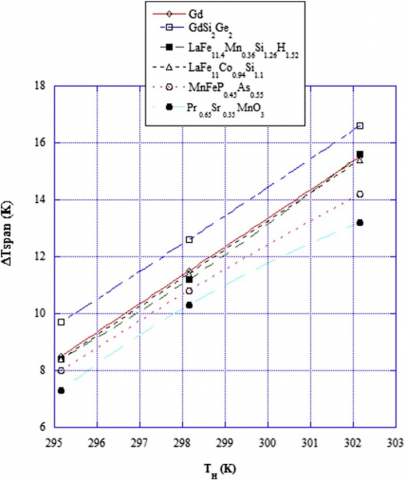
Figure 11 reports ∆Tspan as a function of hot heat exchanger temperature for all the tested material, that have been compared with gadolinium [22].
Figure 11. ∆Tspan as a function of TH [22]
The general trend, as expected from equation (8), shows that the temperature span increases with the increasing hot-side temperature. The greatest values of temperature span are that proper of Gd5(Si2Ge2) (from +7 to +14% with respect to pure Gd), even if the investigated temperature range does not include its Curie point; rather than Pr0.65Sr0.35MnO3 of whom are registered the smallest ΔTspan despite that its Curie temperature is quite centered in the explored temperature range. LaFeSi compounds show value of ΔTspan like Gd ones.
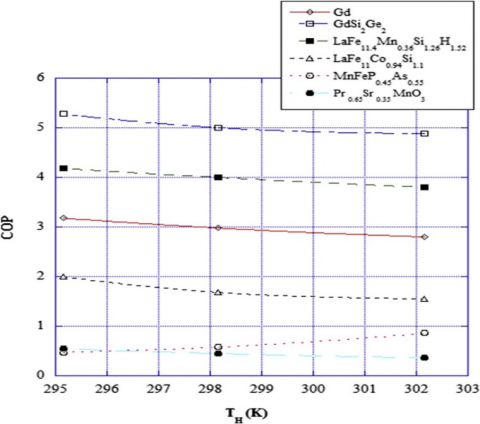
Figure 12 shows coefficient of performance as a function of hot heat exchanger temperature for all the materials above introduced. As visible, COP decreases with the increasing of the amplitude of temperature investigated range. The highest values of COP have been estimated for Gd5(Si2Ge2) since that they are averaging higher than gadolinium of +40%; also in LaFe11.384Mn0.356Si1.26H1.52 it has been registered an increment of +30%, still considering gadolinium as benchmark. On the other side, LaFe11.05Co0.94Si1.10, MnFeP0.45As0.55 and Pr0.65Sr0.35MnO3 always underperform gadolinium.
Figure 12. COP as a function of TH [22]
Several campaigns of numerical simulations have been conducted, through a two-dimensional model of an AMR regenerator. The model, which can reproduce the behavior of the Rotary Permanent Magnet Magnetic Refrigerator built at University of Salerno, has been previously validated with experimental results under two different situations (zero-load and iso-load). Whereupon, a number of campaigns of simulations has been conducted in order to carry out a performance map, which constitute a tool, able to indicate the way to go for the optimization of the prototype. A huge part of the investigation has been devoted to gadolinium, the benchmark refrigerant for magnetic refrigeration, so to explore the limit conditions of prototype working, in terms of cold-hot heat exchanger range, fluid flow rate and frequency. Successively, the performance map has been extended to other materials, possible candidates for refrigeration, revealing that, from an efficiency point of view, the best candidates to magnetic refrigeration is Gd5(Si2Ge2) which exhibits the highest values of ΔTspan and COP but, on the other side, it is a very expensive material, disadvantage which makes it impractical for every economic plan of magnetic refrigerator commercialization. From a global point of view (performances and cost), the most promising materials are LaFeSiH compounds which are cheaper than rare earth materials and compounds, i.e. gadolinium and Gd5(Si2Ge2), and they give performances sufficiently higher to be considered candidates as refrigerant for magnetic refrigeration.
|
B |
magnetic field induction, T |
|
C |
specific heat, J. kg-1. K-1 |
|
G |
gain, K |
|
H |
magnetic field intensity, A. m-1 |
|
k |
thermal conductivity, W. m-1. K-1 |
|
m |
fluid flow rate, kg. s-1 |
|
M |
magnetization, A. m-1 |
|
p |
pressure, Pa |
|
Q |
thermal power, W |
|
S |
entropy, J. K-1 |
|
T |
temperature, K |
|
t |
time, s |
|
u |
longitudinal velocity, m.s-1 |
|
v |
orthogonal velocity, m.s-1 |
|
W |
work, J |
|
x |
longitudinal spatial coordinate, m |
|
y |
orthogonal spatial coordinate, m |
|
Greek symbols |
|
|
Δ |
finite difference |
|
η |
isentropic efficiency |
|
θ |
period of the whole AMR cycle, s |
|
µ |
dynamic viscosity, kg. m-1. s-1 |
|
υ |
cinematic viscosity, m2. s-1 |
|
ρ |
density, kg. m-3 |
|
τ |
period of magnetization/demagnetization process of AMR cycle, s |
|
Subscripts |
|
|
CF |
cold-to-hot flow process |
|
D |
demagnetization process |
|
F |
fluid (pure water) |
|
HF |
hot-to-cold flow process |
|
M |
magnetization process |
|
T |
temperature |
[1] United Nation Environment Program (UN). (1987). Montreal Protocol on substances that deplete the ozone layer, New York, NY, USA.
[2] Mirandola A., Lorenzini E. (2016). Energy, environment and climate: from the past to the future, Int. J. of Heat and Technology, Vol. 34, No. 2, pp. 159-164. DOI: 10.18280/ijht.340201
[3] Aprea C., Greco A., Maiorino A. (2013). The substitution of R134a with R744: an exergetic analysis based on experimental data, Int. J. of Refr., Vol. 36, No. 8, pp. 2148-2159. DOI: 10.1016/j.ijrefrig.2013.06. 012
[4] Greco A., Mastrullo R., Palombo A. (1997). R407C as an alternative to R22 in vapour compression plant: An experimental study, Int. J. En. Res., Vol. 21, pp. 1087-1098. DOI: 10.1002/(SICI)1099-114X(19971010) 21:12<1087::AID-ER330>3.0.CO;2-Y
[5] Kyoto Protocol to the United Nation Framework Convention on Climate Change. (1997). Kyoto, JPN.
[6] Aprea C., Greco A., Maiorino A., Masselli C., Metallo A. (2016). HFO1234ze as drop-in replacement for R134a in domestic refrigerators: An environmental impact analysis, Energy Procedia, Vol. 101, pp. 964-971. DOI: 10.1016/j.egypro.2016.11.122
[7] Aprea C., Greco A., Maiorino A., Masselli C., Metallo A. (2016). HFO1234yf as a drop-in replacement for R134a in domestic refrigerators: a life cycle climate performance analysis, Int. J. of Heat and Techn., Vol. 34, No. Sp. 2, pp. S212-S218. DOI: 10.18280/ijht.34S2
[8] Salata F., Golasi I., Falanga G., Allegri M., de Lieto Vollaro E., Nardecchia F., Pagliaro F., Gugliermetti F., de Lieto Vollaro A. (2015). Maintenance and energy optimization of lighting systems for the improvement of Historic buildings: A case study, Sustainability (Switzerland), Vol. 7, No. 8, pp. 10770-10788. DOI: 10.3390/su70810770
[9] Salata F., Golasi I., di Salvatore M., de Lieto Vollaro A. (2016). Energy and reliability optimization of a system that combines daylighting and artificial sources. A case study carried out in academic buildings, Applied Energy, Vol. 169, pp. 250-266. DOI: 10.1016/j.apenergy.2016.02.022
[10] Mauri L., Carnielo E., Basilicata C. (2016). Assessment of the impact of a centralized heating system equipped with programmable thermostatic valves on building energy demand, Energy Procedia, Vol. 101, pp. 1042-1049. DOI: 10.1016/j.egypro.2016.11.132
[11] Vallati A., Grignaffini S., Romagna M., Mauri L. (2016). Effects of different building automation systems on the energy consumption for three thermal insulation values of the building envelope, EEEIC 2016 – Proceedings of International Conference on Environment and Electrical Engineering, art. no. 7555731.
[12] Mauri L. (2016). Feasibility analysis of retrofit strategies for the achievement of NZEB target on a historic building for tertiary use, En. Proc., Vol. 101, pp. 1127-1134. DOI: 10.1016/j.egypro.2016.11.153
[13] Salata F., Golasi I., de Lieto Vollaro R., de Lieto Vollaro A. (2016). Urban microclimate and outdoor thermal comfort. A proper procedure to fit ENVI-met simulation outputs to experimental data, Sustainable Cities and Society, Vol. 26, pp. 318-343. DOI: 10.1016/j.scs.2016.07.005
[14] Aprea C., Greco A., Maiorino A. (2015). The application of a desiccant wheel to increase the energetic performances of a transcritical cycle, Energy Conversion and Management, Vol. 89, pp. 222-230. DOI: 10.1016/j.enconman.2014.09.066
[15] Kitanovski A., Plaznik U., Tomc U., Poredos A. (2015). Present and future refrigeration and heat pump technologies, Int. J. of Refrig., Vol. 57, pp. 288-298. DOI: 10.1016/j.ijrefrig.2015.06.008
[16] Aprea C., Greco A., Maiorino A., Masselli C. (2017). Electrocaloric refrigeration: an innovative, emerging, eco-friendly refrigeration technique, IOP Conf. Series: Journal of Physics: Conf. Series, Vol. 796, p. 012019. DOI: 10.1088/1742-6596/796/1/012019
[17] Aprea C., Greco A., Maiorino A., Masselli C. (2017). A comparison between electrocaloric and magnetocaloric materials for solid state refrigeration, International Journal of Heat and Technology, Vol. 35, No. 1, pp. 225-234. DOI: 10.18280/ijht.350130
[18] Yu B.F., Liu M., Egolf P.W., Kitanovski A. (2010). A review of magnetic refrigerator and heat pumps prototypes built before the year 2010, Int. J. of Refrig., Vol. 33, No. 6, pp. 1029-1060. DOI: 10.1016/j.ijrefrig.2010.04.002
[19] Aprea C., Greco A., Maiorino A., Masselli C. (2015). Magnetic refrigeration: An eco-friendly technology for the refrigeration at room temperature, Journal of Physics: Conference Series, Vol. 655, No. 1, p. 012026. DOI: 10.1088/1742-6596/655/1/012026
[20] Aprea C., Greco A., Maiorino A., Masselli C. (2017). A two-dimensional investigation about magnetocaloric regenerator design: Parallel plates or packed bed? IOP Conf. Series: Journal of Physics: Conf. Series, Vol. 796, p. 012018. DOI: 10.1088/1742-6596/796/1/012018
[21] Aprea C., Greco A., Maiorino A., Mastrullo R., Tura A. (2014). Initial experimental results from a rotary permanent magnet magnetic refrigerator, Int. J. of Refrig., Vol. 43, pp. 111-122. DOI: 10.1016/j. ijrefrig.2014.03.014
[22] Warburg, E., “Magnetische Untersuchungen. Über einige Wirkungen der Coërcitivkraft Annalen der Physik”, Vol. 13, pp. 141-164, 1881. DOI: 10.1002/andp.18812490510
[23] Walker G. (1983). Claude and Joule-Brayton Systems, The International Cryogenics Monograph Series, ed. Springer, 1983, ch. Cryocoolers, pp. 297-353. DOI: 10.1007/978-1-4899-5286-8_7
[24] Barclay J.A. (1982). The theory of an active magnetic regenerative refrigerator, NASA STI/Recon Technical Report, No. 83, p. 34087.
[25] Blanco J.A., Gignoux D., Schmitt D. (1991). Specific heat in some gadolinium compounds. II. Theoretical model, Phys. Rev. B, Vol. 43, No. 13, pp. 145-151. DOI: 10.1103/PhysRevB.43.13145