OPEN ACCESS
The classical Crane 1970 and Pavlov 1974 problem of a stretching sheet in a Newtonian fluid is extended to effects of porosity, MHD, mass transfer and heat transfer. Analytical solution is obtained for velocity and temperature solutions of the subsequent linear non-homogenous ordinary differential is expressed in terms of confluent hypergeometric function, it is also known as Kummer’s function of first kind. Heat transfer analysis is classified into two types of boundary layer heating process, namely, prescribed surface temperature (PST) as well as prescribed surface heat flux (PHF), both of which are thought to be quadratic functions of distance. The problem has industrial applications in extrusion process and such other allied areas.
MHD, newtonian fluid, stretching/shrinking sheet, porous medium, mass transfer, non-linear differential equation, heat transfer, kummer’s function
Now-a-days, consideration has been given to somewhat novel kind of flow circumferences that has been of the classical laminar boundary layer flows due to a stretching boundary is an important phenomenon because of its wide range of technological applications in polymer extrusion process. Several processes in chemical engineering such as, greasing up oils, multi-review oils, gypsum glues, printer inks, pottery, fluid cleansers, blood, paints, natural product juices, the rates of cooling and stretching highly influence the quality of the final product. of consistent strips, polymers extrusion process involved cooling of molten liquid being stretched into a cooling system, glass- fibers drawn through a quiescent electrically conducting liquid subject to a magnetic field, and the purification of molten metals from nonmetallic inclusions and change their viscosity or flow actions under stress and thus diverge from the conventional Newton’s law of viscosity.
The investigation of steady laminar boundary flows, heat and mass exchange has gotten extensive considerations on account of its expanding mechanical applications furthermore, critical direction on a few mechanical procedures, for example, the production, the drawing of plastics and elastic sheets, the metal and polymer expulsion forms, the glass-fiber, the paper creation, and the cooling of vast metallic sheets in a cooling bath. The streamlined expulsion of plastic sheets, the limit layer along a fluid film in buildup process and a polymer sheet or fiber expelled consistently from a pass on, or a long string going between a feed roll and a wind-up roll are the case of down to earth utilizations of a persistent level surface.
Blasius (1908) firstly discovered the boundary layer flows on a flat plate via similarity transformation. Unique in relation to Blasius, Sakiadis (1961) considered the steady laminar boundary layer flow on a moving level plate in a calm liquid and got numerical arrangement of the issue, furthermore, later the work was reached out to the flow because of stretching of a sheet by Crane (1970). The flow of a viscous fluid past a linear stretching plate is a classical problem in laminar boundary layer flows. Crane (1970), first got an analytical solution to the laminar boundary layer equations for the problem of two-dimensional flow due to a linear stretching plate in a gentle incompressible liquid.
The aim of the present article is to investigate the combined effect of heat source/sink and stress work on MHD Newtonian fluid flow over a stretching porous sheet. The problem is important in its applications to extrusion and stretching problems. The solution also belongs to the rare class of exact similarity solutions of the Navier–Stokes equations.
We consider two dimensional, laminar, steady, boundary layer flow of an incompressible, Newtonian, electrically conducting fluid over a stretching porous sheet in the presence of heat source/sink and stress work as shown in the figure 1.A homogeneous magnetic field apparently exists in the direction perpendicular to the sheet. It is assumed that the changes in the induced magnetic field and the external electric field of MHD because of the polarization of charges are negligible. Considering the above assumptions into account, the Navier-Stokes equations to the steady, laminar and Newtonian boundary layer fluid flow are:
Figure1. Schematic diagram of the stretching boundary
An electrically conducting fluid is penetrated by imposing a consistent field B0, which acts in the vertical direction.The Reynolds number is assumed to be negligibly small.Also, viscous and Ohmic dissipation terms as well as the Hall effect are neglected (see Mahabaleshwar 2008).In considerations of the above, the governing sets of equations are,
$\frac{\partial u}{\partial x}\,+\frac{\partial v}{\partial y}=0$ ,(continuity) (1)
(x-momentum)
$u\frac{\partial u}{\partial x}+v\frac{\partial u}{\partial y}\,=\nu \frac{{{\partial }^{2}}u}{\partial {{y}^{2}}}-\left( \frac{\nu }{K}+\frac{\sigma B_{0}^{2}}{\rho } \right)u,$ (2)
Temperature
$\begin{align} \rho {{C}_{p}}\left( u\frac{\partial t}{\partial x}+v\frac{\partial t}{\partial y} \right)\ =\ \kappa \frac{{{\partial }^{2}}t}{\partial {{y}^{2}}}\,+\left( \frac{\mu }{K}+\sigma H_{0}^{2} \right){{u}^{2}}\,+ \mu \,{{\left( \frac{\partial u}{\partial y} \right)}^{2}}\,+{{Q}_{1}}\left( T-T\infty \right) \\\end{align}$ (3)
The corresponding boundary conditions are as follows:
$\begin{align}\left. \begin{smallmatrix}u=\alpha x,\,\,\text{v}={{\text{v}}_{c}} \\ t={{t}_{\text{w}}}={{t}_{\infty }}+A{{x}^{2}}\,\text{in}\,\text{PST}\\-\kappa \frac{\partial t}{\partial y}={{q}_{\text{w}}}\text{= }B{{x}^{2}}\text{ in}\,\text{PHF}\end{smallmatrix} \right\}\text{at}\,\,y=\text{0,} \\u\to 0,\,\,\,\,\,\,\,t\to {{t}_{\infty }}\,\,\,\,\,\,\,\,\,\,\,\,\,\,\text{as }\,y\to \infty . \\\end{align}$ (4a,b,c,d)
Here, u is the velocity component along the x axis and v is the velocity component along y axis, tw is the temperature of the sheet,t is the temperature of the fluid, t∞ is the temperature of the fluid far away from the sheet,Q1 is the heat source/sink coefficient, $\kappa $ is the thermal conductivity, K is the permiabilty of the porous medium, $\sigma $ is the electricalconductivityofthefluid, ${{C}_{p}}$ is the specific heat at constant pressure, $\rho $ is the density ${{Q}_{1}}$ is the volumemetric rate of heat generation when ${{Q}_{1}}>0$ and heat absorbation when ${{Q}_{1}}<0$ . The axial and transverse velocities at the distances next to the normal surface Equation (3c) implies that the liquid has no lateral motion as $y\to \infty $ . As $y\to \infty $ in Eq.(3c), the stretching sheet does not incite dynamics into the flow at distances moving far away from the sheet.In the present case, the flow due to the stretching of the sheet, which is free from the stream velocity, and also the pressure gradient, is zero.Using the dimensionless variables
$\left. \begin{align} \left( U,V \right)=\frac{\left( u,v \right)}{\sqrt{\alpha \nu }},\left( X,Y \right)=\left( x,y \right)\sqrt{\frac{\alpha }{\nu }} \\ T=\frac{t-{{t}_{\infty }}}{{{t}_{w}}-{{t}_{\infty }}},{{t}_{w}}-{{t}_{\infty }}=\left\{ \begin{smallmatrix}A{{x}^{2}}\text{ }\,\text{in}\,\,\,\,\,\,\,\text{PST} \\\text{ }\frac{\text{B}{{x}^{2}}}{\kappa }\text{ }\,\,\,\,\text{in}\,\,\,\,\,\,\,\,\text{PHF}\end{smallmatrix} \right\} \\\end{align} \right\}$ , (5a,b)
in Eqs. (1)-(3), the following transformed governing equation are obtained:
$\frac{\partial U}{\partial X}\,+\frac{\partial V}{\partial Y}=0$ (6)
$U\frac{\partial U}{\partial X}+V\frac{\partial U}{\partial Y}\,=\frac{{{\partial }^{2}}U}{\partial {{Y}^{2}}}-\left( D{{a}^{-1}}+Q \right)U$ (7)
$\begin{align} U\frac{\partial T}{\partial X}+V\frac{\partial T}{\partial Y}\,=\frac{1}{\Pr }\frac{{{\partial }^{2}}T}{\partial {{Y}^{2}}}-\frac{1}{\Pr }\left( D{{a}^{-1}}+Q \right){{U}^{2}} +E{{\left( \frac{\partial U}{\partial Y} \right)}^{2}}+{{\beta }_{1}}T, \\\end{align}$ (8)
where, $Q={}^{\sigma B_{0}^{2}}/{}_{\alpha \rho }$ is the Chandrasekhar number, $\Pr ={}^{\nu }/{}_{\chi }$ is the Prandtl number, $E={}^{{{\alpha }^{2}}}/{}_{{{C}_{p}}A}$ viscous dissipation parameterand $D{{a}^{-1}}={}^{\nu }/{}_{\alpha K}$ is the inverse Darcy number, ${{\beta }_{1}}={}^{{{Q}_{1}}}/{}_{\alpha \rho {{C}_{p}}}$ is the heat/source sink parameter ${{\beta }_{1}}<0$ .reduces the temperature in the fluid as the effect of source and ${{\beta }_{1}}>0$ enhance the temperature. The effective coolling of the sheet heat sink prefered. The boundary conditions become
$\left. \begin{align} U=X,\,\,V={{V}_{c}},\left\{ \begin{smallmatrix}T=1\,\text{in }\,\text{PST} \\\frac{\partial T}{\partial Y}=-1\,\,\text{in}\,\,\,\,\text{PHF}\end{smallmatrix} \right\}\text{at}\,\,Y=\text{0,} \\ U\to 0,T\to 0\,\,\,\,\,\,\,\,\,\,\,\,\,\,\,\,\,\,\,\,\,\,\,\,\,\,\text{as }Y\to \infty . \\\end{align} \right\}$ (9a, b)
Introducing the physical stream function $\psi \left( X,Y \right)$ to satisy the conservation of massin the dimensionless form (6) , we may write.
$U=\frac{\partial \psi }{\partial Y},V=-\frac{\partial \psi }{\partial X}.$ (10)
Using Eq.(10), Eqs. (7) and (8) , can be written as
$\frac{\partial \psi }{\partial Y}\frac{{{\partial }^{2}}\psi }{\partial X\partial Y}-\frac{\partial \psi }{\partial X}\frac{{{\partial }^{2}}\psi }{\partial {{Y}^{2}}}\,=\frac{{{\partial }^{3}}\psi }{\partial {{Y}^{3}}}-\left( D{{a}^{-1}}+Q \right)\frac{\partial \psi }{\partial Y}$ (11)
$\begin{align} \frac{\partial \psi }{\partial Y}\frac{\partial T}{\partial X}-\frac{\partial \psi }{\partial X}\frac{\partial T}{\partial Y}\,=\frac{1}{\Pr }\frac{{{\partial }^{2}}T}{\partial {{Y}^{2}}}-\frac{1}{\Pr }\left( D{{a}^{-1}}+Q \right){{\left( \frac{\partial \psi }{\partial Y} \right)}^{2}} +Ec{{\left( \frac{{{\partial }^{2}}\psi }{\partial {{Y}^{2}}} \right)}^{2}}. \\\end{align}$ (12)
The corresponding boundary condition (9) interms of the physical stream function takes in the fom
$\begin{align} \frac{\partial \psi }{\partial Y}=X,\,\,\frac{\partial \psi }{\partial X}={{V}_{c}}\left\{ \begin{smallmatrix} T=1\,\,\,\,\text{in }\,\text{PST} \\ \frac{\partial T}{\partial Y}=-1\,\,\,\,\text{in}\,\,\,\,\text{PHF}\end{smallmatrix} \right\}\,\text{at}\,\,Y=\text{0,} \\ \frac{\partial \psi }{\partial Y}\to 0,T\to 0\,\,\,\,\,\,\,\,\,\,\,\,\,\,\,\,\,\,\,\,\,\,\,\,\,\,\,\,\,\,\,\,\,\,\,\,\,\,\text{as }Y\to \infty . \\\end{align}$ (13)
In order to to convert the system of nonlinear partial differential equations (11) and 12) into highly nonlinear ordinary differential equations the following similarity tranformation is used
$\psi \left( X,Y \right)=X\,f\left( \eta \right),\,$
$T\left( X,Y \right)=\left\{ \begin{align} & \theta \left( \eta \right)\,\,\,\text{in}\,\text{PST} \\ & \phi \left( \eta \right)\,\,\,\,\text{in}\,\text{PHF} \\ \end{align} \right\},$ (14)
$\eta =Y$ (15)
Substitution of Eq. (14) and (15) in Eq. (11) and results in the following nonlinear ordinary differential equation with constant coefficient:
${{f}_{\eta \eta \eta }}-f_{\eta }^{2}+f\,{{f}_{\eta \eta }}-\left( D{{a}^{-1}}+Q \right){{f}_{\eta }}=0$ (16)
where the subsripts denotes differentiation with respect to the similar ity variable $\eta .$ The corresponding boundary conditions given by Eqs. (13) to be satisfied by f can be obtained for velocity in the form
$f\left( 0 \right)={{V}_{c}}$ , ${{f}_{\eta }}\left( 0 \right)=1$ , ${{f}_{\eta }}\left( \infty \right)=0$ . (17)
In equation (16), the combined effect of Chandrasekhar number Q and the inverse Darcy number $D{{a}^{-1}}$ results in the linear drag force, which acts against the flow of the fluid and this opposition due to porous medium and the MHD is known as Darcy drag and Lorentz Drag respectively.This drag force is of much advantageous as this reduces the effect of two parameters into one.We now, search the solution of the laminar boundary value problem (16) and (17) in the following closed analytical form,
$f\left( \eta \right)={{V}_{C}}+\left[ \frac{1-Exp(-\beta \eta )}{\beta } \right]$ (18)
where, $\beta >0$ must satisfy the quadratic equation,
${{\beta }^{2}}-{{V}_{c}}\beta -\left( 1+Q+D{{a}^{-1}} \right)=0$ (19)
$\beta =\frac{{{V}_{c}}\pm \sqrt{{{V}_{c}}^{2}+4\left( 1+Q+D{{a}^{-1}} \right)}}{2}$ (20)
where, ${{V}_{c}}={}^{{{v}_{c}}}/{}_{\sqrt{\alpha \nu }}$ represents the suction/injection parameter(mass transpiration) and three cases arises depending on the choice of ${{V}_{c}},$ namely suction, impermeable and injection when ${{V}_{c}}>0$ , ${{V}_{c}}=0$ and ${{V}_{c}}<0$ respectively.
Using Eq.(12) in Eq.(13), we get the following boundar value problems
PST case
${{\theta }_{\eta \eta }}+\Pr \,f\,{{\theta }_{\eta }}-\Pr \left( 2\,{{f}_{\eta }}-{{\beta }_{1}} \right)\theta =-Pr\,E\,\left\{ f_{\eta \eta }^{2}+\left( Q+D{{a}^{-1}} \right)f_{\eta }^{2} \right\}$ (21)
$\begin{align} \theta =1\,\,\,\,\,\,\,\,\,\,\,\,\,\,\,\,\,\,\,\,\,\text{at}\,\,\,\,\,\,\,\,\,\,\,\,\,\eta =0, \\ \theta \to 0\,\,\,\,\,\,\,\,\,\,\,\,\,\,\,\,\,\,\text{as}\,\,\,\,\,\,\,\,\,\,\,\eta \to \infty . \\\end{align}$ (22)
PHF case
${{\phi }_{\eta \eta }}+\Pr \,f\,{{\phi }_{\eta }}-\Pr \left( 2\,{{f}_{\eta }}-{{\beta }_{1}} \right)\phi =-Pr\,E\,\left\{ f_{\eta \eta }^{2}+\left( Q+D{{a}^{-1}} \right)f_{\eta }^{2} \right\}$ (23)
$\begin{align} {\phi }'=-1\,\,\,\,\,\,\,\,\,\,\,\,\,\,\,\,\,\text{at}\,\,\,\,\,\,\,\,\,\,\,\,\,\eta =0, \\ \phi \to 0\,\,\,\,\,\,\,\,\,\,\,\,\,\,\,\,\,\,\text{as}\,\,\,\,\,\,\,\,\,\,\,\eta \to \infty . \\\end{align}$ (24)
Figure 2a.Variation of horizontal velocity (f) for different values of the Chandrasekhar number(Q) and inverse Darcy number(Da-1) when Vc = 0.1.
Figure 2b.Variation of axial velocity (fɳ) for different values of the Chandrasekhar number(Q) and inverse Darcy number(Da-1) when Vc = 0.1.
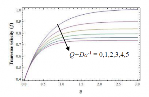
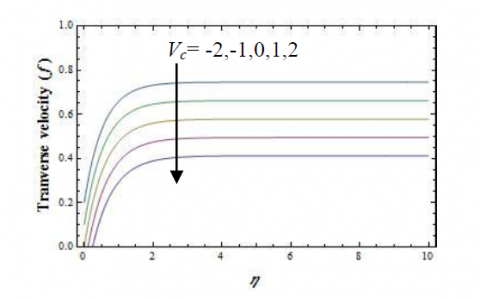
Figure 3a.Variation of transverse velocity (f) for different values of the suction/injetion parametre VcwhenQ +Da-1=1.
Figure 3b.Variation of axial velocity (fɳ)) for different values of the suction/injetion parametre Vc whenQ +Da-1 =1.
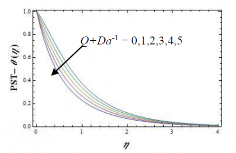
Figure 4a.Variation of heat transfer PST $\theta (\eta )$ for different values of the Q+ Da-1 when Vc = 0.1, Pr=1 andE= 0.1and ${{\beta }_{1}}=0.01$
Figure 4b.Variation of heat transfer PHF $\theta (\eta )$ for different values of the Q+ Da-1 when Vc = 0.1, Pr=1 andE= 0.1and ${{\beta }_{1}}=0.01$
The analytical solutions of equations (21) - (24) are obtained and the solutions are analyzed graphically for different values of Eckert number, Chandrasekhar number, inverse Darcy number, Prandtl number and mass transpiration parameter andinternal heat generation.Now, another type of heating process, namelyprescribed heat flux is considered as it is better suited for effective cooling of the stretching sheet.The results are shown graphically.
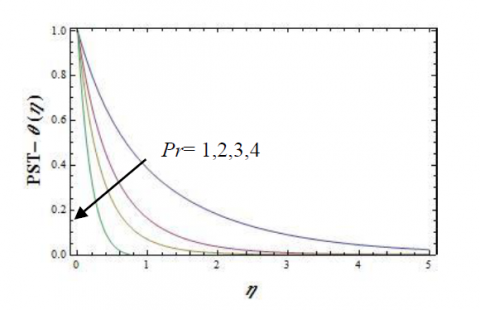
Figure 5a.Variation of heat transfer PST $\theta (\eta )$ for different values of the Prwhen Vc = 0.1, Q+ Da-1=1 andE= 0.1and ${{\beta }_{1}}=0.01$
Figure 5b.Variation of heat transfer PHF $\phi (\eta )$ for different values of the Prwhen Vc = 0.1, Q+ Da-1=1 andE= 0.1 and ${{\beta }_{1}}=0.01$ .
Figure 6a.Variation of heat transfer PST $\theta (\eta )$ for different values of the viscous dissipation parameter EQ+Da-1 = 1when Vc = 0.1, Pr=1 and ${{\beta }_{1}}=0.01$ .
Figure 6b.Variation of heat transfer PHF $\phi (\eta )$ for different values of the viscous dissipation parameter EQ+Da-1 = 1when Vc = 0.1, Pr=1
The outcomes from the exact analytical solutions of the velocity and temperature in the sheet are obtainable for all independent parameters of the Newtonian fluid over the plate, as unraveled by Eqs. (16), (17),(21),(22),(23) and (24).The variations of velocity components along and in the axial direction of the sheet aredisplayed at Figs. 2a and 2b for different combined of values ofQ+Da-1, the Chandrasekhar number and inverse Darcy number.
Figures 2a,b and 3a,bdipicts the two velocity profile distributions, ${{f}_{\eta }}$ and $f\left( \eta \right)$ i.e. the velocity components u and v at the axial and transversedirections, respectively, versus $\eta $ for various values of theQ+Da-1abd mass transfer Vc.Since the present review is a speculation of the established works of Crane [7] and Pavlov (1974) their answers are likewise introduced in both figures. The present outcomes approach asymptotically the consequences of Crane (1970) as $Q\to 0$ ,furthermore, the consequences of Pavlov (1974) $D{{a}^{-1}}\to 0$ and $D{{a}^{-1}}\to 0$ Gupta and Gupta (1977).
In addition, distributions of temperature are displayed at Figs. 4 to 6 for a range of values of Prandtl(Pr), Eckert E, the Prandtl, combined Chandrasekhar-Darcry (Q+Da-1) numbers are studied individually.Together to the flow components of the Newtonian liquid, heat transfer from the sheet is additionally vital.The main conclusions derived from the present investigation can be listed as follows:
|
$c$ |
constants rate of stretching (s-1) |
|
A, B, C |
constants |
|
${{B}_{0}}$ |
magnetic field (T-Tesla) |
|
E |
viscous dissipation |
|
Da-1 |
inverse Darcy number |
|
f |
similarity function for velocity |
|
k |
thermal conductivity |
|
Pr |
Prandtl number |
|
Q |
Chandrasekhar’s number |
|
${{Q}_{1}}$ |
internal heat generation |
|
t |
fluid temperature |
|
u, v |
velocity components along x&y-axis (m s-1) |
|
U, V |
dimensionless velocity components along x and y-axis (m s-1) |
|
${{v}_{w}}$ |
mass transpiration parameter |
|
${{V}_{c}}$ |
dimensionless mass transpiration parameter |
|
x, y |
axial and transverse axes (m) |
|
Greek letters |
|
|
$\alpha $ |
constant |
|
$\mu $ |
viscosity (kg m-1s-1) |
|
$\theta $ |
dimensionless temperature in PST case |
|
$\phi $ |
dimensionless temperature in PHF case |
|
$\rho $ |
density (kgm-3) |
|
$\sigma $ |
electrical conductivity |
|
$\nu $ |
kinematic viscosity, $\left( ={\mu }/{\rho }\; \right)$ (m2 s-1 ) |
|
$\kappa $ |
permeability parameter |
|
$\psi $ |
physical stream function (m2 s-1 ) |
|
Subscripts |
|
|
0 |
pole |
|
w |
wall condition |
|
$\infty $ |
far from the sheet |
|
${{f}_{\eta }}$ |
first order derivative with respect to $\eta $ |
|
${{f}_{\eta \eta }}$ |
second order derivative with respect to $\eta $ |
|
${{f}_{\eta \eta \eta }}$ |
third order derivative with respect to $\eta $ |
[1] Abramowitz M., Stegun F. (1980). Handbook of mathematical functions, Dover, New York.
[2] Blasius H. (1908). Grenzschichten in FlüssigkeitenmitkleinerReibung, Z. Angew. Math. Phys.(ZAMP), Vol. 56, pp. 1–37.
[3] Crane L.J. (1970). Flow past a stretching plate, ZAMP21, pp. 645-647. DOI: 10.1007/BF01587695
[4] Chaim T.C. (1997). Magnetohydrodynamic heat transfer over a non-isothermal stretching sheet, Acta Mech., Vol. 122, pp. 169–179. DOI: 10.1007/BF01181997
[5] Pavlov K.B. (1974). Magnetohydrodynamic flow of an incompressible viscous liquid caused by deformation of plane surface, Magnetnaya Gidrodinamica, Vol. 4, pp. 146-147. DOI: 10.22364/mhd
[6] Mahabaleshwar U.S. (2013). Linear stretching sheet problem with suction in porous medium Open Journal of Heat, Mass and Momentum Transfer, Vol. 1, No. 1, pp. 13-18. DOI: 10.12966/hmmt.07.02.2013
[7] Gupta P.S., Gupta A.S. (1977). Heat and mass transfer on a stretching sheet with suction or blowing, Can. J. Ch. Eng, Vol. 55, pp. 744-746. DOI: 10.1002 /cjce. 5450 550 619
[8] Carragher P., Crane L.J. (1982). Heat transfer on a continuous stretching sheet, ZAMM, Vol. 62, p. 564. DOI: 10.1002/zamm.19820621009
[9] Nield D.A., Bejan A. (2013). Convection in Porous Media, 4th Edn. Springer, New York. DOI: 0-1772415-3260-0-9781475730333
[10] Fisher E.G. (1976). Extrusion of Plastics, (3rd Edition. Newnes-Butterworld, London. DOI: 10.2478/ijame-2013-0059
[11] Sakiadis B.C. (1961a). Boundary-layer behavior on continuous solid surfaces I: The boundary layer on an equation for two dimensional and axisymmetric flow, AIChE J., Vol. 7, pp. 26-28. DOI: 10.1002/aic.690070108
[12] Sakiadis B.C. (1961b). Boundary-layer behavior on continuous solid surfaces II: The boundary layer on a continuous solid surface, AIChE J., Vol. 7, p. 221. DOI: 10.1002/aic.690070211
[13] Sakiadis B.C. (1961c). Boundary-layer behavior on continuous solid surfaces III: The boundary layer on a continuous cylindrical surface, AIChE J., Vol. 7, p. 467. DOI: 10.1002/aic.690070325