OPEN ACCESS
The use of passive safety systems are more and more diffused in many technological fields. Natural circulation is probably one of the main phenomenon applied in this kind of systems: indeed, as known, by means of gravity and buoyancy forces, the fluids can circulate without any external power sources. In this paper, a preliminary analysis (also by comparisons between experimental tests and numerical simulations) of a natural circulation based loop (namely a natural circulation based facility installed at University of Genova) is presented. Starting from some experimental results, the data deriving from CFD loop simulations (both in steady and in unsteady conditions) are used for a first preliminary validation, mainly in order to have a computational tool reliable and able to computationally simulate motion inversions related phenomena. The physical inversions phenomena are very well reproduced also by the a simplified numerical 2D model of the loop, and the physical considerations related to the temperature and velocity fluctuations during the transient simulations, are in agreement with the well-known observations formulated by Welander on the basis of a simple point source analysis scheme.
CFD, natural circulation, ansys-fluent, single phase, rectangular loop
Natural circulation applied to energy systems is widely analyzed by international agencies and research groups. This phenomenon plays a very important role in all the applications that need passive safety systems, and, for its intrinsic applicability features (it is a natural passive methodology), it is the basis of many traditional and innovative technologies.
Particularly, as a significant example, new developments in nuclear applications (e.g. GEN-IV plants) need to have a deep overview on the passive safety systems applied to research [13] and power [3] installations. As past nuclear accidents teach, the safety of nuclear systems is strongly related to their cooling systems, not only during normal operation, but for the whole time the nuclear fuel is contained in the plant. Therefore, the use of passive systems is one of most important issues in new nuclear applications. As known, up to 7% of the full thermal power is provided by a nuclear power plant also after its shutdown: there is, namely, an important power rate that has to be extracted by the coolant even after the plant has been shut down. A lot of studies have been carried forward on this topic (e.g., the IAEA provided several investigations about natural circulation applied to advanced water cooled reactors [6]). However, this paper does not want to analyze a specific type of NPP, but it would be a contribution to the application of natural circulation in the design of a key component present in many nuclear installation, namely the Decay Heat Removal (DHR) system. In fact, as known, those systems have to dispose the decay heat during the shutdown in the case of active cooling systems failures. Without neutron flux increase (i.e. no criticality insertions), DHRs are characterized by a well-defined thermal flux to be extracted, and they have to be self-sustainable (i.e. passively operated, also without external power sources) from cooling point of view.
So, in order to have adequate tool for simulating innovative reactors behaviors, we chose to (preliminarily) validate a numerical analysis by a CFD code (namely ANSYS FLUENT 14 [1]) on an experimental facility that could simulate a natural circulation regime typically found in an advanced nuclear reactor, similarly to what already done for developing some innovative components (e.g. [4][7]).
2.1 Experimental apparatus
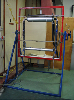
The experimental apparatus consisted of a rectangular loop with the heater on the bottom and the heat exchanger on the top. Fig. 1 shows a picture of the loop. The two vertical tubes were insulated by means of an Armaflex® layer of 2 cm thickness (l = 0.038 W/m∙K at 40 °C) and they can be considered adiabatic. At the heating section, a controllable heat flux was imposed before, and a controllable temperature at the cooling section later. The vertical tubes and the four bends were made of stainless steel AISI 304, while the horizontal tubes were made of copper.
Figure 1. Experimental natural circulation loop [9]
For the entire loop, the internal diameter D was 30 mm; the loop height (H) was 0.988 m and the total length Lt, measured on the tube axis, was 4.100 m, with a Lt/D ratio of 136.7.
The heater was constructed from an electrical Nicromel wire rolled uniformly around the copper tube, and connected to a programmable power supply (Sorensen DHP 150-33). On the upper part of the loop a coaxial cylindrical heat exchanger was connected to a cryostat (Haake KT90): this one was able to maintain a constant temperature of -20 °C of the cooling medium with a cooling power of 1 kW, and constant temperatures ranging from -10 °C to +30 °C with a cooling power of 2.5 kW. The coolant flowing through the annulus was a 50% water/glycol mixture, with a freezing point of -40 °C. An external pump was needed in order to achieve maximum flow rate of 2 m3/h; this was needed to maintain the temperature difference of less than 1 °C between inlet and outlet section of the heat exchanger. This requirement formed the practical definition of constant temperature for the heat sink. Both heater and cooler were thoroughly insulated. Experimental tests and CFD simulations [10] demonstrated that heat loss from the heater to the environment were lower than 5% of the total heat flux.
An open expansion tank connected to the top of the loop allowed the working fluid to expand as its temperature increased, while keeping atmospheric pressure inside the loop.
It is necessary to point out that, even though the experimental apparatus can operate in a wide range of parameters, for the numerical analysis performed in this paper it has been considered only a single value for the thermal power (2000 W) and for the heat sink temperature (20 °C).
All the calibrated thermocouples (±0.1 °C) used in this apparatus were T-type with external diameters of 0.5 mm. As shown in Fig. 2, twenty thermocouples measured the fluid temperature in the 4 sections (from A to D), placed 142 mm far from the nearest horizontal side axis. In each section one thermocouple was located on the vertical tube axis, while the other 4 were radially placed at a distance of D/4 from the tube wall and circumferentially distributed at each 90°.
Figure 2. Thermocouples siting
The temperatures at the inlet and outlet sections of the secondary flow of the heat exchanger were evaluated by the two thermocouples 27 and 28 in Fig. 2. The internal temperature of the cryostat was also measured by thermocouple, and two thermocouples were positioned at the top and the bottom of the loop in order to check any changes in the room temperature. In addition, eighteen thermocouples were placed inside the heater insulation in order to investigate natural circulation phenomena in porous media [10]. Again, Fig. 2 shows the general siting of the thermocouples used.
Experimental data were acquired over a period of 21600 seconds (6 hours) and stored by mean of a high-speed data acquisition system (National Instruments PCI-1200, SCXI-1000, SCXI-1102, SCXI-1303). The acquisition time interval was 1 second and each data item was the average of 1000 readings per second.
The loop was designed to accommodate different inclinations, to reduce the buoyancy forces and simulate reduced gravity [12]. However, for the present study, experiments were performed only with the vertical configuration.
Table 1. Water properties
|
ρ |
991 |
kg/m3 |
|
β |
400.4∙10-6 |
K-1 |
|
µ |
631∙10-6 |
kg/m∙s |
|
cp |
4.178 |
kJ/kg∙K |
|
Pr |
4.16 |
- |
The water properties, evolving inside the loop, evaluated at 42 °C (average water temperature obtained as a result of experimental tests), numerically implemented by the Boussinesq approximations, are reported in Tab. 1.
The loop hydraulic diameter and height are respectively 0.03 m and 0.988 m.
The cooler evolving fluid is, as already anticipated, a 50% water + 50% glycol mixture whose properties (evaluated at 10 °C [8]) are shown in Tab. 2.
Table 2. Water-glycol (50%-50%) mixture properties
|
ρ |
1084 |
kg/m3 |
|
µ |
2.7∙10-3 |
kg/m∙s |
|
Cp |
3.28 |
kJ/kg∙K |
|
Pr |
21.8 |
- |
2.3 Experimental procedures
Even if in the present paper only a heat power over 2000 W and heat sink temperature of 20 °C was numerically compared with the corresponding experimental data, the procedures adopted during the considered experiments was the same employed in several experimental campaigns previously performed [11].
Before starting each run, the temperature of the internal bath of the cryostat was set to the test value. This was necessary, because the cryostat contained approximately 85% of the coolant of the system, the rest being inside the upper heat exchanger and the connections. Then, the “stagnant” condition (i.e. when the temperature differences between all thermocouples in the fluid were lower than 0.5 °C) was checked. Each run was started by simultaneous initiation of data acquisition, power supply and cooling flow. The operating parameters were maintained constant for 6 hours, when the run was terminated by switching off the power supply and cryostat, and stopping the data acquisition.
This procedure caused a limited transient period in the secondary flow (shorter than 10 minutes). This period is necessary for the cryostat to control the coolant fluid amount (15%) present in the upper heat exchanger.
3.1 Numerical models
Figure 3. 3D computational fluid domain
The numerical simulation of the natural circulation loop has been performed in two consecutive steps; the first one involved a 3D complete loop geometrical domain and a stationary solver, in order to calculate a reasonable value of the cooler-side convective heat transfer coefficient by changing the temperature value at the cooler.
The second step involves a 2D fluid domain with transient solver and using the heat transfer coefficient value calculated by previous 3D model, with the aim of evaluating the fluid dynamics behavior inside the loop and verify numerically the proper expected flow reversal phenomena observed during the experiments. The 3D computational domain is reported in Fig. 3.
3.2 3D steady-state simulations
The 3D computational domain includes the whole loop internal volume and the solid region of the pipes and junction elements (in order to include also the thermal capacity effects of the materials by means of a conjugate heat transfer model); the full 3D model of the cooler is implemented, too.
The imposed ANSYS FLUENT Boundary Conditions (BCs) referred to Fig. 3, are:
Starting from the BCs above reported, the complete stationary heat transfer process has been evaluated, neglecting only the unsteady terms.
Second order Upwind numerical interpolation scheme was used for T, v, k and ε equations; instead, for pressure equation, the Body Force Weighted scheme was used.
With the value reported in the previous Tab. 1, we can calculate the Rayleigh number by modified Grashof number of the loop, as indicated in [14][15]:
$G{{r}_{m}}=\frac{{{D}^{3}}{{\rho }^{2}}\beta gPH}{A{{\mu }^{3}}{{c}_{p}}}$ (1)
and consequently
$Ra=G{{r}_{m}}\Pr =1.154\cdot {{10}^{15}}$ (2)
Considering this very high value of Ra, the natural fluid motion are fully turbulent inside the loop.
Looking at the numerical turbulence models, for steady-state analyses with SIMPLE pressure-velocity coupling scheme, we chose a RNG k-ε turbulence model with enhanced wall treatment.
Finally, the solid body materials properties, like aluminum for the clamp components and steel for the legs and other pipes, are those implemented in the ANSYS-FLUENT 14 material database.
In the following, the results of a sensitivity mesh analysis were presented; then a preliminary 3D test will be performed with the selected grid, by varying the heat power at the heater and the heat sink temperature, with the aim of investigating the relations between the heat sink temperature and the Nu number on the cooler-side. The obtained relation will be used for the HTC cooler-side imposition in the 2D transient simulations.
3.2.1 Grid sensitivity analysis
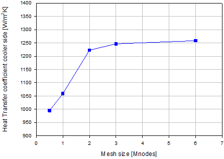
In order to avoid grid errors, a grid independency analysis has been performed with 0.5, 1, 2, 3 and 6 millions of nodes; the results are reported in fig. 4 and tab. 3, in which the HTC values for the cooler are evaluated as
$HTC=\frac{{{P}_{heater}}}{{{A}_{cooler}}\Delta T}$ (3)
where:
• Acooler is the internal surface of heat exchange (i.e. the external loop pipe surface enclosed by the cooler volume)
• ΔT is the difference by the mean temperature of the same surface and the Heat Sink (HS) imposed temperature
Table 3. Numerical results of grid independency test (P = 2000 W, THS = 20 °C)
|
Mesh_size [Mnodes] |
T_surface [°C] |
HTC [W/m2∙K] |
ΔTcooler [°C] |
T_bulk [°C] |
v_bulk ·101[m/s] |
|
0.5 |
44.2 |
995.6 |
1.1 |
66.6 |
1.2 |
|
1.0 |
42.9 |
1059.0 |
1.1 |
63.6 |
1.0 |
|
2.0 |
40.1 |
1222.8 |
1.1 |
60.0 |
0.8 |
|
3.0 |
39.7 |
1246.9 |
1.1 |
58.2 |
0.8 |
|
6.0 |
39.1 |
1253.5 |
1.1 |
58.0 |
0.8 |
Figure 4. Grid independency HTC results
3.2.2 HTC analysis
As a consequence of the previous sensitivity analysis, the grid selected for the final run has 3 million of tetrahedral cells. The maximum Aspect Ratio and Skewness are 5 and 0.85 respectively.
Considering the mesh independency analysis performed, the HTC value obtained was compared to two semi-empiric correlations [2], namely:
• Dittus-Boelter:
$Nu=0.023{{\operatorname{Re}}^{0.8}}{{\Pr }^{0.4}}$ (4)
• Churchill-Bernstein:
$\begin{align} Nu=0.3+ \frac{(0.62 {{\operatorname{Re}}^{0.5}}{{\Pr }^{0.33}})}{{{\left[ 1+{{\left( \frac{0.40}{\Pr } \right)}^{0.66}} \right]}^{0.25 }} }{{\left[ 1+{{\left( \frac{\operatorname{Re}}{282000} \right)}^{0.625}} \right]}^{0.8}} \\\end{align}$ (5)
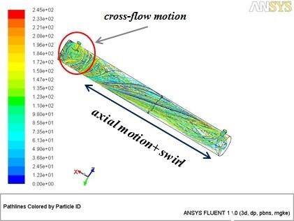
Churchill-Bernstein (Eq. 5) and Dittus-Boelter (Eq. 4) correlations have been chosen due to the nature of the fluid motion inside the cooler, depicted in Fig. 5: As it can be seen in the geometrical section near the inlet, the motion is fully cross-flow; instead in the other portion of the cooler the fluid have an axial motion distorted by a low frequency swirl component.
Figure 5. Pathlines water-glycol mixture inside cooler
The comparison performed (Tab. 4 shown the value obtained with THS = 22 °C and P = 2000 W) shows that, as expected, each correlation predicts a different value: due to the hybrid nature of motion, the Churchill-Bernstein correlation predicts a higher value, instead Dittus-Boelter underestimates the value calculated by ANSYS-FLUENT.
Table 4. HTC comparison at THS = 22 °C
|
Correlations |
HTC_cooler [W/m2∙K] |
|
ANSYS-FLUENT |
1264 |
|
Dittus-Boelter |
249 |
|
Churchill |
4796 |
Due to this significant difference between HTC values calculated by CFD and semi-empirical correlations, 9 numerical 3D simulations (varying the power levels at the heater and the heat sink temperatures) were carried out. The obtained results are shown in Fig. 6: the heat sink temperature seems to have some influence; instead it seems possible to neglect the power level at the heater dependency.
Starting from the obtained results, a simple but ad-hoc correlation (where the water-glycol mixture properties could be calculated on the basis of the heat sink imposed temperature) was obtained by a correlation that, in the considered Re range, gives results similar to linear regression (Fig. 7):
$Nu=5.2+1.4{{\operatorname{Re}}^{0.444}}$ (6)
The Reevaluation was based on the material properties of the water-glycol at different heat sink temperature and the velocity in the inlet pipe. The dependency of Re by the heat sink temperature is bound to the water-glycol properties dependency, as summarized in Tab. 5.
Figure 6. HTC vs. heat power and heat sink temperature (calculated by ANSYS FLUENT 3D simulations)
Table 5. Water-glycol properties dependency by temperature
|
HS_T [°C] |
ρ [kg/m3] |
Cp [J/kg∙K] |
μ [kg/m∙s] |
v [m/s] |
Re_D [-] |
|
-10.0 |
1094.0 |
3201.0 |
5.3E-03 |
21.6E-02 |
2.8E+04 |
|
0.0 |
1090.0 |
3240.0 |
3.7E-03 |
21.6E-02 |
4.4E+04 |
|
10.0 |
1084.0 |
3280.0 |
2.7E-03 |
21.8E-02 |
6.1E+04 |
|
22.0 |
1079.0 |
3321.0 |
2.0E-03 |
21.9E-02 |
8.2E+04 |
Figure 7. HTC specific correlation
The HTC value calculated by the proposed correlation (Eq. 6) will be used as a convective boundary conditions in the 2D transient simulations reported in the next paragraph.
3.3 2D transient simulations
Due to the high computational resources required for a 3D transient simulation, it was created a 2D domain extrapolated by the 3D mid-section without the cooler volume, as shown in Fig. 8. The grid is structured with 106 nodes (due to a high wall refinement). The BCs and numerical scheme set are the same of the 3D simulations; only the cooler was set differently, namely as wall with convective and conductive heat transfer.
The temporal discretization is a Second Order Implicit type and the time step was chosen equal to 10-3 s, in order to obtain a Courant number smaller than 1.
Adopting the presented setting, the calculations time (by a parallel 4-way solver, i.e. a quadcore i5 processor, 2.3 GHz) has been about 35 days.
Figure 8. 2D domain and particular of structured grid
The comparison between CFD and experimental results was carried out at 2000 W of heater power and 8 °C of heat sink temperature.
In Fig. 9 a comparison between the mean temperature measured inside the loop and that one calculated by ANSYS FLUENT in the mean vertical section of the legs is reported.
Figure 9. Experimental vs. CFD mean temperature comparison
The results show a very good agreement both in term of temperature value and curve trend. There are many point of motion inversion; CFD calculations predict a lower temperature value with an average deviation of 10%; only in the final part (i.e. for time longer than 800 s) of the test (not reported in Fig. 9), the experimental results show a relative stabilization of the motion without inversions, differently from CFD calculations where the motion keeps an unstable behavior.
Fig. 10 shows the average velocity in the middle section of the loop’s legs: analyzing the velocity, it is clear that not for each temperature inversion corresponds an effective flow reversal phenomenon. In some case the velocity magnitude decreases until a zero gradient point with a minimum value, then the magnitude increases and, at the next decreasing period, follows the flow reversal.
Figure 10. Average velocity in the middle section of the loop's legs
One of the most important CFD result is reported in fig. 11 (the scales in the figure are arbitrary modified and dimensionless in order to “overlap” the curves). The phase shift between the curves, and in particular, the velocity “delay” (with respect to the temperature) in the left leg are relevant and can play an important role in the inversion phenomena, as further explained in the follow.
Figure 11. Temperature and velocity normalized trend (scales modified for overlapping the curves)
The measured Δp between the two legs (due the inversion of the fluid motion during the experiments, each leg is alternately the “cold” or the “hot” leg, so each one represents alternatively positive and negative value of the pressure drop) and the temperature differences are detailed reported in [5].
During the experimental test, the friction factor “f” has been evaluated by the Colebrook’s correlation while the velocity has been evaluated by means of pressure drop expressed by the following equation:
$\Delta p=\frac{1}{2}\frac{{{L}_{tot}}}{D}f\rho {{v}^{2}}$ (7)
where Ltot takes into account the localized 90° curve pressure drop.
Then, due the relations between the pressure drop and the velocity (see Eq. 7), the velocities calculated with ANSYS-FLUENT (shown in Fig. 11) are representative of the experimental pressure drops.
As shown by Welander’s analysis [16] performed by a theoretical calculation with a point sources (Fig. 12-A), the nature of the inversion of the motion are produced by a phase displacement between flow rate and total buoyancy force (fig. 12-B); the same observation could be done looking at both the experimental [5] and the CFD calculations results (Fig. 11), where the velocity characterizes the flow rate and the temperature the buoyancy force.
Figure 12. Welander’s theory: (A) calculation scheme and (B) results graphic representation [5][16]
Natural circulation is a spontaneous phenomenon that occurs when in a fluid gravity and buoyancy forces are established. This passive behavior can be exploited through closed loops in order to extract the heat from a source and to yield it to a sink. Here some experimental and numerical analyses on a closed rectangular loop built at DIME/TEC - University of Genova are shown.
In the present paper, the comparison between experimental data and numerical simulations are presented. The commercial solver ANSYS-FLUENT 14 was employed to develop both a 2D and a 3D models. The latter model was applied in the case of steady-state conditions and its results, in terms of HTC at the cooler, where used in the 2D transient model.
The numerical models take explicitly into account the pipes and insulation material, with the clamp component simulated with an equivalent volume for the correct consideration of the heat capacity contribution above all in the transient calculations.
Generally speaking, there is a good agreement between the experimental and numerical results.
The obtained numerical simulations, in accordance with Welander’s point source theory, reproduce correctly the phase displacement between the flow rate and total buoyancy force.
Finally, even in a relatively simple geometry, the required computational effort results to be quite significant for the transient simulations, due to the high number of cells necessary for the solid pipe material and the very low time step required by the Courant-Friedrichs-Lewy conditions [2].
As future developments, other unsteady simulations will be performed with finer grid and Large Eddy Simulations turbulence models with the main aim of analyzing more in detail the phenomenology of the inversion of the motion. Additionally, also 3D unsteady simulations would be useful, provided that enough computational resources will be available.
First of all, we like to thank Ing. D. Traverso for his fundamental past contribution to this research activity. Furthermore, we want to thank Dr. Ing. R. Marotta of Nucleco S.p.A. for his support. Finally, we want to thank Dr. F. Magugliani of Ansaldo Nucleare S.p.A. for his precious suggestions and help with computational related issues.
|
Δp |
Pressure difference, [Pa] |
|
ΔT |
Temperature difference, [K] or [°C] |
|
A |
Surface, [m2] |
|
Cp |
Specific heat, [kJ/kg∙K] |
|
D |
Diameter, [m] |
|
f |
Friction factor, [-] |
|
H |
Height, [m] |
|
HTC |
Heat Transfer Coefficient, [W/m2∙K] |
|
NPP |
Nuclear Power Plant |
|
p |
Pressure, [Pa] |
|
P |
Power, [W] |
|
T |
Temperature, [K] or [°C] |
|
v |
Velocity, [m/s] |
|
L |
Length, [m] |
|
Grm |
Modified Grashof number |
|
Nu |
Nusselt number |
|
Pr |
Prandtl number |
|
Ra |
Rayleigh number |
|
Re |
Reynolds number |
|
Greek symbols |
|
|
β |
Thermal expansion coefficient, [K-1] |
|
l |
Thermal conductivity, [W/m∙K] |
|
µ |
Dynamic viscosity, [Pa∙s] |
|
ρ |
Density, [kg/m3] |
|
k |
Turbulent kinetic energy, [m2/ s2] |
|
ε |
Turbulence dissipation, [m2/ s3] |
|
ω |
Turbulence dissipation rate, [s-1] |
[1] ANSYS (2011). Fluent 14.0 User’s Guide.
[2] Bejan A., Kraus A. D. (2003). Heat Transfer Handbook, John Wiley & s.
[3] Cerullo N., Lomonaco G. (2012). Generation IV reactor designs, operation and fuel cycle, Nuclear Fuel Cycle Science and Engineering, pp. 333-395, Woodhead Publishing. DOI: 10.1533/9780857096388.3.333, 2012.
[4] Ferrini M., et al. (2015). Design by theoretical and CFD analyses of a multi-blade screw pump evolving liquid lead for a Generation IV LFR, Nucl. Eng. Des., Vol. 297, pp. 276-290. DOI: 10.1016/j.nucengdes.2015.12.006
[5] Garibaldi P. (2007). Single-phase natural circulation loops: Effects of geometry and heat sink temperature on dynamic behaviour and stability, Ph.D. Thesis, tutor: Misale M., Università degli Studi di Genova.
[6] IAEA (2012). Natural circulation phenomena and modelling for advanced water cooled reactors, IAEA-TECDOC-1677, from http://www-pub.iaea.org/books/IAEABooks/8638/Natural-Circulation-Phenomena-and-Modelling-for-Advanced-Water-Coolied-Reactors, accessed on 25 Aug.2017.
[7] Mangialardo A., et al. (2014). Numerical investigation on a jet pump evolving liquid lead for GEN-IV reactors, Nucl. Eng. Des., Vol. 280, No. C, pp. 608-618. DOI: 10.1016/j.nucengdes.2014.09.028
[8] Melinder A. (2007). Thermophysical properties of aqueous solutions used as secondary working fluids, Ph.D. Thesis, Royal Institute of Technology (KTH).
[9] Misale M., et al. (2011). Influence of thermal boundary conditions on the dynamic behaviour of a rectangular single-phase natural circulation loop, Int. J. of Heat and Fluid Flow, Vol. 32, pp. 413-423. DOI: 10.1016/j.ijheatfluidflow.2010.12.003
[10] Misale M., et al. (2007). Experiments in a single phase natural circulation mini-loop, Exp. Therm. and Fluid Sci., Vol. 31, pp. 1111-1120. DOI: 10.1016/j.expthermflusci.2006.11.004
[11] Mousavian S.K., et al. (2004). Transient and stability analysis in single-phase natural circulation loop, Ann. Nucl. Energy, Vol. 31, pp. 1177-1198. DOI: 10.1016/j.anucene.2004.01.005
[12] Misale M., Marasso M., Devia F. (2003). Numerical simulation of a single-phase natural circulation loop for different gravitational fields, XXI Congress UIT sulla Trasmissione del Calore, Udine, Italy, UIT03-324.
[13] Ripani M., et al. (2014). Study of an intrinsically safe infrastructure for training and research on nuclear technologies, European Physical Journal - Web of Conferences, Vol. 79, No. 02004. DOI: 10.1051/epjconf/20137902004.
[14] Vijayan P.K. (2001). Experimental observations on the general trends of the steady state and stability behavior of single-phase natural circulation loops, Nucl. Eng. Des., Vol. 215, pp. 139-152. DOI: 10.1016/S0029-5493(02)00047-X
[15] Vijayan P.K., et al. (2001). Investigations of the effect of heater and cooler orientation on the steady state, transient and stability behaviour of single-phase natural circulation in a rectangular loop, Bhabha Atomic Research Centre, India, report number: 2001/E/034.
[16] Welander P. (1967). On the oscillatory instability of a differentially heat fluid loop, Fluid Mechanics, Vol. 29, pp. 17-30. DOI: 10.1017/S0022112067000606