OPEN ACCESS
Energy consumption in buildings is a relevant international topic driving policy measures for energy saving. In this context the Energy Efficiency Directive are mainly focused on the new building construction and renewable energy resources exploitation.
On the other hand the potential of new buildings in Europe is very limited, if compared to existing buildings. Therefore the major part of primary energy savings can be expected from optimized exploitation and refurbishment of already installed, conventional heating systems.
Even if a good solar energy fraction can be exploited by means of solar panel installation, energy savings can also be obtained by means of smart control of existing heating plants (thermostatic control valves).
This work in particular focuses on the possibility to use simplified approaches for the analysis of energy savings that can be obtained adjusting the heating system control, using current energy sources and plants.
To this aim a simplified dynamic numerical code has been developed using EES (Engineering Equation Solver) to simulate both the building physics and the heating system, coupled to each other. This model was applied to some building case studies to identify in each case the best heating system control criteria and qualify the corresponding energy saving achievements.
Building heating system, Dynamic simulation, Energy savings, Smart regulation and control.
The global increase of energy demand has assumed a great international importance in view of the CO2 emission reduction. Buildings are responsible of about 40 % of the total energy consumption [1], therefore it is important to enhance they energy performance. The growing trend in heating and cooling energy demand causes a relevant concern on the adequate development of energy system and energy policies [2]. In the building context energy is consumed for different final uses, such as DHW (domestic hot water), lighting, and electric appliances, but space heating is indeed the dominant energy end use. Energy efficiency is a valuable means to address this problem and improves the Union’s security of supply by reducing the primary energy consumption and decreasing energy import [3].
Heating and cooling is the largest single source of energy demand in Europe and the majority of Europe’s gas imports are used for these purposes. Huge efficiency gains remain to be captured with regard to district heating and cooling, which will be addressed in a Commission strategy [4].
The European Council of March 2007 emphasized the need to increase energy efficiency in the Union so as to achieve the objective of reducing by 20% the Union’s energy consumption by 2020 and called for thorough and rapid implementation of the priorities established in the Commission Communication entitled “Action plan for energy efficiency: realizing the potential”. This action plan identified the significant potential for cost-effective energy saving in the buildings sector [5]
Several numeric models were developed over the years to simulate the energy performances of buildings. Generally steady state approaches [6,7] are commonly used to estimate the building consumption in the preliminary stage of the design or for scenario analyses. In the last years, researchers have performed and compared a lot of dynamic numerical models, in order to analyze their capability in predicting the energy demand of buildings. Boyer et al.[8] introduced the nodal analysis for determining the thermal behavior of buildings: considering a one-dimensional conduction across the walls and introducing their thermal capacities, each building component (wall, heating zone, etc.) was modeled as a node in which the energy conservation law is applied.
Hudson and Underwood[9] tested a thermal model based on a lumped-capacity treatment of the building elements adopting the electrical analogy. The model has been applied to a building with high thermal capacity, showing a good agreement between numerical and experimental results. They concluded that there are no advantages in using a higher-order description of walls if short-term transient analyses are considered.
Nielsen [10] developed a simple tool to evaluate building energy demand in a transient context. The simulator is based on the lumped capacitance approach and a unique heating zone is considered. The equation system consists in two differential equations, one for the internal air and the other for all the opaque structures grouped into a single effective capacitance. Moreover, an algebraic equation is added to account for the conduction across the walls and the solar contribution in the internal surfaces.
On the other hand, most of the new technologies based on the building thermal inertia can be modelled only by transient thermal models. Moreover, transient simulation play a fundamental role to propose optimal energy saving solutions, especially in the short time regulation criteria, which assume an important role in the global energy performance of energy integrated system [11].
Even if several dynamic calculation software are available for the space heating energy demand evaluation (MC4, TRANSYS, ENERGY PLUS, and so on) most of them are rather difficult to be used when facing the retrofitting of existing plants (e.g. ECOTEC applications in [12]).
This paper focuses on simplified methods able to explain dynamic energy building consumptions and trends, when different control strategies are applied for the heating system operation in dynamic conditions. The aim is global building energy assessment methodologies based on bottom-up analyses, instead of “top-down” ones, based on statistical or global screening methods, such as the one developed in [13].
The building physics are formulated in a mathematical method implemented in EES (Engineering Equation Solver) [7]. The aim is to design a control strategy able to minimize the energy consumption, while guaranteeing that all comfort requirements are met.
In order to quantify the internal comfort as a result of the time history of local temperature values, some new roper comfort and energy performance parameters are proposed and defined as a time integration of the main operating temperatures and temperature gradients, in order to understand how much each energy saving achievement affects comfort results during the building operation.
The most important design parameters of the building affecting indoor thermal comfort and energy conservation in building are included, even if only a trend analysis is performed, since important data such as site and orientation, and windows deployment are neglected.
Indeed such data affects actual energy needs of the building, but the dynamic behaviour and potential energy savings coming from smart regulation are mainly affected by the building aspect ratio, thermo-physical proprieties of the building envelope and heating energy system installed.
2.1 Heating zone
A building physics model was created to represent heat transfer between the building and the outside environment. The model is developed to test the thermal control outcomes of a building, with reference to some standard configuration.
The reference configuration here assumed is the one usually adopted for the calculation of mean building energy needs (EN 11330).
The dynamic model describes the energy and mass balance of air in the building having a heating system. The main purpose of the model is not to emulate future reconstruction or design for a new building, but improve the heating system regulation in existing buildings, looking for “optimized control”. The building is modelled as a single isothermal air volume with a unique thermal capacity (Figure 1).
Figure 1. Schema of the internal volume modelling
This volume exchanges heat with the internal wall layers and receives heat by heating elements and by internal free gain by internal heat sources (persons, equipment and lighting).
The transient energy balance equation for the internal air A-node can be written as in Eq. (1):
$(M C)_{A} \cdot \frac{d T_{A}}{d \tau}=Q_{H S}-Q_{A, I}-Q_{A, P}+Q_{s o u r c e}$(1)
QHS is the heating input thermal power from heating elements
QA,I represents the heat exchange with the internal walls and furniture
QA,P represent the heat losses through the external walls
Qsource represent the internal heat source due to persons, equipment and appliances.
The internal air temperature TA is one of the main comfort parameters, together with thermal gradients with cold walls on the external part of the envelope.
2.2 External walls
All the external walls are modeled as a unique node temperature TP with its related thermal capacitance. The 3-node model is used to simulate dynamic heat transfer between the wall and the adjacent environment (Figure 2). Two different layers are considered: the internal layer (at inside temperature TPI), which exchanges heat with the internal mass of air, and the external one (at the external wall temperature TPE), which is subjected to the combined effect of external air convection and solar irradiation. The dynamic wall temperature is assumed to be the one of the central node, TP.
Figure 2. Schema of the external wall modelling
The transient energy balance equation for opaque external wall can be written as in Eq. (2)
$(M C)_{P} \cdot \frac{d T_{P}}{d \tau}=\dot{Q}_{P, i}-\dot{Q}_{P, e}$(2)
The where (MC)P is the wall thermal capacity and TP is the node temperature of the wall. Moreover QP,i represent the heat flux of the internal wall towards the inner wall surface Ai,E, QP,e represent the heat flux of the external wall towards the external wall surface AE (both of them represented by means of an inside thermal resistances RP,i; RP,e respectively).
The energy balance equation for the external and internal wall node temperature can be expressed using the following equation:
$Q_{P, i}=A_{i, E} \cdot \frac{T_{P, i}-T_{P}}{R_{P, i}}$(3)
$Q_{P, e}=A_{E} \cdot \frac{T_{P}-T_{P, e}}{R_{P, e}}$(4)
The internal surface wall temperature TP,I is used to calculate the internal heat transfer with the ambient air at TA (assumed to be just convective, for simplicity), while the external wall surface temperature TP,E is used in the calculation of the external surface heat balance, which includes convection and radiation with the external environment and solar irradiation on horizontal surface (G) in the daylight period. Qrad is the solar radiation contribution on the vertical surface, which depends on G and on the wall orientation
$h_{i, E} \cdot\left(T_{A}-T_{P, i}\right)=\frac{T_{P, i}-T_{P}}{R_{P, i}}$(5)
$\frac{T_{P}-T_{P, e}}{R_{P, e}}+\frac{Q_{R A D}-Q_{E}}{A_{e}}=0$(6)
$Q_{E}=A_{e}\left[h_{E}\left(T_{P, e}-T_{E}\right)+\sigma \varepsilon_{T}\left(\left(T_{P, e}+273\right)^{4}-\left(T_{E}+273\right)^{4}\right)\right]$(7)
2.3 Radiant heating system
The radiant heating system are modelled considering a single unit element with a thermal capacitance defined as the sum of all elements in the building (Figure 3).
The transient energy balance equation for the radiant heating system can be written as follows:
$(M C)_{H S} \cdot \frac{d T_{H S}}{d \tau}=Q_{W, H S}-Q_{H S}$(8)
$Q_{W, H S}=h_{W, H S} \cdot A_{W, H S}\left(T_{W}-T_{H S}\right)$(9)
$Q_{H S}=h_{H S} \cdot A_{H S}\left(T_{H S}-T_{A}\right)$(10)
where hHS is heat global heat transfer coefficient of the radiant heating system.
Figure 3. Model of the radiant heating system
A thermostatic mixing valve can be installed in the heater element with the aim to vary the mass flow rate flowing in the element according to measured internal air temperature Equation (11). The dynamic response of the thermostatic valve is determined by varying the parameter β in the calculation of δTA, according to Eq(12).
$\dot{M}_{W}=\max \left[0 ; \dot{M}_{W, r i f} \cdot \frac{1}{\sqrt{\left(1+\delta T_{A}\right)}}\right]$(11)
$\delta T_{A}=\max \left[\frac{1}{\Delta M_{\max }^{2}}-1 ; \beta\left(T_{A}-T_{A}^{*}\right)\right]$(12)
where ṀW [kg/s] is the actual flow rate of water flowing through the valve, depending on the valve aperture b and on the nominal water flow rate of the valve, ṀWrif [kg/s], ΔM2max is the maximum percentage of mass flow rate variation, and T*A is the set point environment temperature giving rise to satisfactory comfort of the inside air.
The variation of the mass flow rate as function of β is shown qualitatively in Figure 4 (% of the nominal flow rate in the heating element as a function of the over-temperature of the internal environment in respect of o given set point temperature, for beta=1, 10 , 100). As it can be seen, the flow rate goes rapidly to zero as soon as the temperature excess is high, but is also suddenly completely opened as soon the ambient temperature is lower than the set point one.
Different simulation curves can be obtained changing the design β values.
Figure 4. Variation of mass flow rate against aperture parameter β, due to the action of the thermostatic valve.
2.4 Heating system
The heating system considered in the present work is an instantaneous response boiler with an ON/OFF regulation criteria. The water temperature at the exit of the heating unit TC is considered to be constant and equal to 65°C. The main components considered in the system model are show in Figure 5. The control action is performed by a mixing valve based on the external temperature, with a setting curve shown qualitatively in Figure 6, defining the outlet flow temperature set point T*M required by the system as function of the temperature difference between a reference temperature (e.g. 20°C) and the external temperature, TE.
$T_{M}^{*}=\operatorname{Min}\left(T_{C} ; \overline{T}_{A}+\alpha \cdot\left(\overline{T}_{A}-\overline{T}_{E}\right)\right)$(13)
2.5 Comfort sensation indexes
The purpose of this section is to investigate the problem of determining a human thermal sensation index that can be automatically calculated and used as feedback control of the heating system. Indeed thermal comfort and energy efficiency seems to be contrasting operating objectives, therefore some compromise must be chosen, that is to design a heating control system that can guarantee high performance (energy savings) while assuring satisfactory comfort (high values of the comfort parameters).
Figure 5. Schema of heating system
Figure 6. Mixing valve characteristic profile
Research has shown that it is possible to reach these objectives if the heating system control strategies are based on thermal sensation index instead of air temperature values alone.
An essential requirement for continued normal body function is that deep body temperature will be maintained within a very narrow limit of ± 1°C, and the discomfort feelings are linked to the efforts the body must devote, by means of internal metabolism, to compensate for external temperature variations. To take into account this point of view integral values over time are needed, rather than simple actual environmental temperature values.
We present a new approach based on three indexes, to estimate the thermal comfort level depending on the state of the following variables: the ambient temperature, the set point ambient temperature, the thermal gradient temperature. All of these three parameters must be integrated over the heating period, to obtain a mean value similar to degree days, but able to express comfort feelings of the body.
The idea is to define an internal discomfort degree days DDTA- coupled to internal and external discomfort index. If the house was not used (that is letting the user to live outdoor) the user should have been subjected to external environment, thus having a discomfort index IBTE-. The use of the house, properly heated, will decrease such discomfort to acceptable values, quantitatively described by the parameter IBTA- assuming that no house at all exist, thus obliging the user to live outdoor.
$D D_{T A}^{-}=\frac{\int \delta T_{A} \cdot d \tau}{24\left[\frac{h}{d a y}\right]}$(14)
$I B_{T A}^{-}=\sqrt{\frac{1}{\tau} \int\left(\min \left(0 ; T_{A}-T_{A}^{*}\right)^{2}\right) d \tau}$(15)
$I B_{T E}^{-}=\sqrt{\frac{1}{\tau} \int\left(\min \left(0 ; T_{E}-T_{A}^{*}\right)^{2}\right) d \tau}$(16)
Since TA* is the environment temperature giving rise to satisfactory comfort (used as the set point), the discomfort integral value is not increased if the actual temperature value is higher than TA*. In other words the value of DDTA- is always negative. A zero value means that the ambient temperature was exactly at the set point all over the time.
2.6 Energy performance parameter
The energy performance parameter equation can be written as follows:
$I P E_{n o m}=\frac{Q_{H, n o m}}{A_{S}}$(17)
$I P E=\frac{Q_{C}}{A_{S}}$(18)
where QH,nom is the nominal heating energy demand of the building and AS is the usable floor area of the building, QC is the actual primary energy consumption, calculated by means of integration during plant operations.
The building here analyzed is a simple parallelepiped with a form factor S/V = 0,6 m-1. This building is modelled as a unique heated zone. The description of geometry and thermophysical proprieties are reported in Table 1.
The numerical model the wall structure must be duly described, the main characteristics of the wall are reported in Table 2.
Several simulations have been conducted in order to test the behavior of the numerical model. In particular the model testing for various thermostatic valve characteristic and for different types of mixing valve regulation of the heating system was performed.
Table 1. Geometric data of the building. S/V=0.6
|
Data |
Units |
Value |
|
Height |
m |
10 |
|
Length |
m |
10 |
|
Width |
m |
10 |
|
Wall transmittance |
W/m2K |
0,329 |
|
Surface mass |
kg/m2 |
379 |
|
Total dissipating surface |
m2 |
600 |
|
Volume |
m3 |
1000 |
|
S/V |
m-1 |
0,6 |
Table 2. Characteristics of the wall structures
|
|
s |
λ |
ρ |
Wall Mass |
R |
U |
|
Units |
m W/(m K) kg/m3 kg/m2 K/W W /m2K |
|||||
|
Internal plaster |
0.02 |
0.700 |
1400 |
28 |
0.029 |
|
|
Air Brick |
0.08 |
0.590 |
1600 |
128 |
0.136 |
|
|
Insulation board |
0.05 |
0.040 |
30.00 |
1.50 |
1.125 |
|
|
Vapour barriers |
0.06 |
0.048 |
33.00 |
1.98 |
1.250 |
|
|
Air Brick |
0.12 |
0.590 |
1600 |
192 |
0.203 |
|
|
External plaster |
0.02 |
0.700 |
1400 |
28 |
0.029 |
|
|
Total |
0.36 |
|
|
379 |
3.04 0.329 |
|
Referring to equations (3,4) a standard ratio Rp,i/Rp,e=0.25
In order to investigate the effect the regulation criteria provided by the mixing valve and the thermostatic valve, a parametric analysis is conducted by varying the parameters β and α, that describe the different response to heating system to the energy demand.
The following figure shows the calculated indoor air temperature TA obtained by varying the parameters α and β.
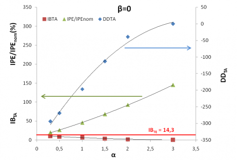
Figures 10, 11, and 12 represents the behavior of thermal sensation indexes and energy consumption parameter (IPE) on the variation of α and β.
The simulations show that the $D D_{T A}^{-}$ Degree days discomfort index depends on a, that is the adaptive capacity of the heating system temperature to the external temperature, but do not depends very much on β.
Figure 7. Temperature profile for β=0 (no thermostatic valves)
Figure 7 shows the results with β=0 and the air temperature to varying α=0,5; α=1; α=1,5; α=2; α=3. When β=0 the heating system is regulated only by means of the mixing valve and the thermostatic valves are not used. So this is the traditional configuration that was used before the installation of thermostatic valves. Figure 7 reports the range of α examined, therefore the consumption needs are estimated according the thermal sensation index and the fluctuations of the indoor temperature.
If α=3 the system response is almost immediate in respect of external temperature variations, so the control does not maintain the right indoor air and creates a fluctuation in temperature equal to the external one (but mirrored, orange line). This behavior highlights that energy consumption for heating will be higher because the indoor temperature shows a considerable increase of temperature that deviates from the average value of the temperature fixed with the set point.
The effects of a reduction of the value of α (2,1.5, 1,…) are a decrease in the indoor temperature and a decrease in the consumption (due to lower internal temperatures). Furthermore, the curves have a lower fluctuation.
The value of a able to give satisfactory results is around 1.5 (purple line).
Figure 8. Temperature profile for β=10 (See Figure 4)
Figure 8 shows the results with β=10 for the air temperature calculations, for values α=0,5; α=1; α=1,5; α=2; α=3. In these simulations the air temperature is mainly driven by the set point of the automatic thermostatic valve. This valve maintains an indoor temperature approaching the temperature of 22°C. The presence of the thermostatic valves makes the building air temperature almost independent of the mixing valve settings, and therefore the parameter α is less important.
Figure 9. Temperature profile for β=500
Figure 9 reports the effect of the increase up to β=500 on the variation of internal air temperature and, as a consequence, on the variation of energy consumption. With β=500 the fluctuation of temperature are even more restricted in the order of ± 1°C with a good tolerance for any α value.
Instead the $I B_{T A}^{-}$ Standard deviation internal discomfort index depends on both α and β, with an higher dependence on α values. Even if it is always lower than the reference value IBTE- =14.3, referring to the “living outdoor” condition, IBTA- values decrease rapidly with α, reaching acceptably low values for α=2 or higher.
The energy consumption parameter IPE of equation (18) increases fast with α, as soon as discomfort parameters reaches acceptable values, but is is strongly affected by the thermostatic valve response time linked to b: as soosn as the response time of the valve becomes very quick, the energy consumption reaches small fractions of the standar energy consumption parameter IPENOM (which is in this case around 110kWh/m2year).
Figure 10. Thermal sensation indexes and energy performance (IPE) for β=0
Figure 11. Thermal sensation indexes and energy performance (IPE) for β=10
Figure 12. Thermal sensation indexes and energy performance (IPE) for β=500
A simplified building dynamic model has been developed and implemented in EES, in order to perform several analyses on heating system in a wide range of regulation conditions.
The analysis shows that a high potential is available to decrease the energy consumption of the building, reducing energy performance index from maximum values of 27 kWh/m2/month down to minimum values of 5 kWh/m2/month. At the same time, however, the discomfort indexes becomes critical, thus suggesting intermediate values of IPE around 15 kWh/m2/month, showing an energy saving of about 16% in respect of standard IPE data of the building of 18.2 kWh/m2/month.
The simulation results show also that when the building was not equipped with a thermostatic valve for the heating elements, the mean temperature was far from the temperature set point, while when the building was supplied with thermostatic valves the overheating was reduced and indoor temperature oscillations where reduced too, thus improving indoor comfort and reducing energy consumption.
In particular the effects of the different regulation settings of mixing valve (α) and thermostatic valve (β) are calculated quantitatively and proven to be extremely different. In the first case (β=0) the thermostatic valves are not used and the internal temperature has some significant fluctuations from the temperature of set point, strongly depending on α values.
Extending the analysis to increasing values of β the building reduce the fluctuations of temperature and reduce also heating energy demand.
Further developments are expected in the definition of proper comfort indexes for the indoor operation, in order to quantify correctly the potential energy savings due to smart regulation for building heating system.
|
A |
area [m2] |
|
C |
thermal capacitance [J K-1] |
|
cp DD H IB IPE M |
water specific heat [J kg K-1] degree days heat transfer coefficient [K W-1] temperature standard deviation [K] energy performance parameter [kWh/m2] water flow rate [kg s-1] |
|
Q R T U |
heat transfer rate [W] thermal resistance [K W-1] temperature [K] transmittance [W m-2 K-1] |
|
Greek symbols |
|
|
a |
parameter of mixing valve |
|
β |
parameter of thermostatic valve |
|
τ |
time [s, h] |
|
σ |
Stefan-Boltzmann constant [W m-2K-4] |
|
Subscripts |
|
|
A |
ambient |
|
E d |
external day |
|
HS i P RAD source W |
heating system internal wall solar radiation internal sources water |
[1] Europe’s Buildings under the Microscope. Buildings Performance Institute Europe (BPIE), 2011
[2] M. Isaac, D.P. Van Vuuren (2009) Modelling global residential sector energy demand for heating and air conditioning in the context of climate change. Energy Policy 37, pp. 507-521.
[3] Directive 2012/27/EU of the European Parliament and of the Council of 25 October 2012 on energy efficiency, amending Directives 2009/125/EC and 2010/30/EU and repealing Directives 2004/8/EC and 2006/32/EC Text with EEA relevance.
[4] Final communication on A Framework Strategy for a resilient Energy Union with a Forward-Looking Climate Change Policy. Energy Union Communication COM, 2015.
[5] The Energy Performance of Buildings (Recast), Council of the European Parliament 2010/31/EU, 19 May 2010.
[6] Energy Conservation in New Building Design, ASHRAE Standard 90A-1980. (Atlanta American Society of Heating Refrigerating and Air Conditioning Engineers)
[7] S.A. Klein, EES - Engineering Equation Solver, F-Chart Software, (2015) Version 9.902, info@fchart.com .
[8] H. Boyer, J. P. Chabriat, B. Grondin-Perez, C. Tourrand and J. Brau, “Thermal building simulation and computer generation of nodal models,” Building and Environment, vol. 31, no. 3, pp. 207–214. DOI: 10.1016/0360-1323(96)00001-7.
[9] G. Hudson and C. P. Underwood, “A simple modeling procedure for Matlab/Simulink,” Proceedings of the IBSPA Building Simulation. Kyoto, pp. 776–83, 1999.
[10] T. Nielsen, “Simple tool to evaluate energy demand and indoor environment in the early stages of building design,” Solar Energy, vol. 78, pp. 73-83, 2005.
[11] Energy Performance of Buildings – Calculation of Energy Use for Space Heating and Cooling, UNI EN ISO 13790:2008. (CEN, UE).
[12] M. Cucumo, V. Ferraro, D. Kaliakatsos and V. Marinelli, (2013). Simulation of the thermal behaviour of buildings equipped with low-emissivity glazed components. Int J Heat & Tech. [Online]. 31(2), pp. 111-118, 2013. DOI: 10.18280/ijht.310215. Available: http://www.iieta.org/Journals/H%26TECH/ARCHIVE/Volume%2031%20No%202
[13] G. Cannistraro, M. Cannistraro and R. Restivo. (2013). Simulation of the thermal behaviour of buildings equipped with low-emissivity glazed components. Int J Heat & Tech. [Online]. 31(2), pp. 155-158. DOI: 10.18280/ijht.310221. Available: http://www.iieta.org/Journals/H%26TECH/ARCHIVE/Volume%2031%20No%202