OPEN ACCESS
The air conditioning of indoor environments requires compliance with the thermo-hygrometric conditions of comfort which also includes the air distribution. This work deals with the thermo-fluid dynamics of the main components of air-conditioning systems, namely primary air systems with fan coils and displacement systems examined in winter and summer conditions. The study highlights the problems of each typology and identifies some best plant solutions. The air distribution systems by means of fan coils allow to reach thermal comfort even at very low speeds, which results also in reduced noise in the environment.
The displacement system allows to work with lower air mass flow rate especially in summer cooling (the reduction is around 60%), whereas slightly different situation occurs in winter conditions. It has been found that it is possible to obtain a flow rate reduction of about 50% by combining together heating and cooling, with a considerable energy savings. The paper shows also that further advantages of the displacement systems compared to an all-air system, has to do with the air velocity values in the occupied space.
Mixing air Distribution, Fan coil, Displacement Systems, Thermal comfort, CFD analysis.
The air distribution in air-conditioned environments is an important issue for thermal comfort. The primary air with fan coil systems and the displacement systems are among the most widely used air-conditioning schemes. Usually the assessment of air distribution requires the use of CFD codes that require a lot of time and computing resources. These tools are justified only in important plant applications such as theaters, museums, exhibition rooms, surgery rooms, etc.
Aim of this paper is to discuss a CFD simulation for the most usual type environments (for example offices) with the two types of systems mentioned above in order to obtain simple practical rules for the system design.
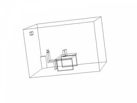
The reference room is of 5 x 4 x 3 m, with thick walls of 0,31 m, openings of 1 x 2.5 m, as shown in Figure 1. Furniture is typical of an office with a chair, a desk and a computer, see Figure 2 and Figure 3.
Figure 1. The reference room
Figure 2. Chair and desk
Figure 3. The reference room with chair and desk inside
The Transfer Function Method (TFM) gives a winter and summer thermal loads which for climatic conditions typical of Sicily for winter and summer respectively is 670 W and 1350 W.
The total air mass flow to be introduced by means of the fan coil is 0.056 m³/s in winter and 0.109 m³/s in the summer. The ventilation flow rate is equal to 11.7 L/s or 42 m³/h.
The primary air is fed with a nozzle of 0.2x0.65 m in size, as shown in Figure 4.
Figure 4. Size and shape of the inlet air nozzle and the fan coil
The wall transmittance is 0.441 W/(m².K) and the windows transmittance is 2.937 W/(m².K). The multi-physical problem involves solution of the conservation laws for mass, momentum, energy and concentration. Under assumptions of Newtonian fluid and uncompressible turbulent flow, the averaged Navier-Stokes equations read as:
$\rho \frac{\partial \mathbf{u}}{\partial t}+\rho(u \square \nabla) \mathbf{u}=\nabla \cdot\left[-p l+\mu\left(\nabla \mathbf{u}+(\nabla \mathbf{u})^{T}\right)-\frac{2}{3} m(\nabla \cdot \mathbf{u}) l\right]+\mathbf{F}$
$\frac{\partial \rho}{\partial t}+\nabla \cdot(\rho \mathbf{u})=0$
$\rho C_{p} \frac{\partial T}{\partial t}+\rho C_{p} \mathbf{u} \cdot \nabla T=Q+k \nabla^{2} T$
The COMSOL Multiphysics® CFD simulation code was utilized. The air and other material properties are shown in table 2.
Figure 5. The mesh of the model
Continuous equations have been spatially discretized by a finite element approach based on the Galerkin method on non-uniform and non-structured computational grids made of triangular Lagrange elements of order 2. Influence of spatial discretization has been preliminary studied in order to assure mesh-independent results, figure 5.
The global flux across the walls in winter is -750 W, the air temperature from the fan coil is 30 °C, the primary air temperature is 20 °C (neutral conditions), the body temperature of the man inside the room is 36 °C and the computer temperature is supposed to be 50 °C. In summer conditions the wall flux is 1000 W, the air temperature from the fan coil is 18 °C, the primary air temperature is 26 °C (neutral conditions).
The simulation was carried out under the hypothesis that the external temperature is sinusoidal with a period of 24 h. The attenuation and phase factor are calculated according ISO EN 13786 for the type of wall used in the model. The parameters for the simulation are summarized in the following tables:
Table 1. Dynamic parameters wall-innner air for the calculation
|
Parameter |
Value |
|
Tm winter |
5 °C |
|
T winter |
10 °C |
|
Tm summer |
25 °C |
|
T summer |
13 °C |
|
Material |
(kg/m³) |
Cp (J/(kgK)) |
k (W/(m K)) |
|
Air |
patm/RT |
1005 |
0.028 |
|
Chair |
30 |
1400 |
0.04 |
|
Body |
985 |
3550 |
0.60 |
|
Equa-tion |
Inlet |
Outlet |
fluid/solid |
External walls |
|
1 |
u=Uin |
p=patm |
U=0 |
U=0 |
|
3 |
T=Tin |
$-\mathbf{n} \cdot(-k \vec{\nabla} T)=0$ |
- |
$-\mathbf{n} \cdot(-k \vec{\nabla} T)$$=h\left(T-T_{e x t}\right)$ |
|
Parameter |
Value |
Units |
|
Thermal flux to the floor |
-200 |
W |
|
Thermal flux for internal wall |
-150 |
W |
|
Fan coil air temperature |
30 |
°C |
|
Primary air temperature |
20 |
°C |
|
Man temperature |
36 |
°C |
|
Computer temperature |
50 |
°C |
|
Parameter |
Value |
Units |
|
Thermal flux to the floor |
-200 |
W |
|
Thermal flux for internal wall |
-150 |
W |
|
Fan coil air temperature |
18 |
°C |
|
Primary air temperature |
26 |
°C |
|
Man temperature |
36 |
°C |
|
Computer temperature |
50 |
°C |
4.1 Fan coil system with primary air
The results for the case of primary air with fan coil system, are summarized in the following figures.
Figures 6 to 9 refer to winter condition, whereas figures 10 to 11 refer to summer conditions.
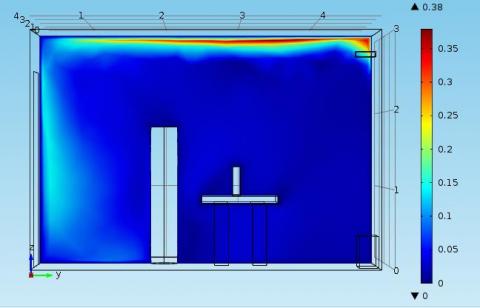
Figure 6. Air Velocity distribution in winter
Figure 7. Air Velocity distribution nearby the human body in winter
Figure 8. Air Velocity distribution in summer
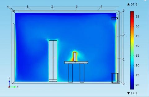
Figure 9. Temperature distribution nearby the human body in winter
Figure 10. Air Velocity distribution nearby the human body in summer
Figure 11. Temperature distribution nearby the human body in summer
The temperature distribution at the head and at the feet of the occupant for winter and summer condition are given in figures 12 and 13.
Figure 12. Air temperature at head and feet in winter
Figure 13. Air temperature at head and feet in summer
On the basis of these results, one can make the following remarks. The primary air and fan coil systems are very simple and reliable. They allow optimal air distribution inside the rooms and make to reach easily the thermal comfort conditions, even at very low speeds. The low speed in turn reduces the noise in the environment.
The use of thicker walls (from 0.331 m to 0.443 m) may allow an easier management of the plant, reducing the energy consumption.
4.1 Displacement system
The second type of plant is the displacement system. The equations to be solved are similar to those already shown. A standard k ε − turbulence model (Launder and Spalding 1974; Ignat et al. 2000) has been applied to solve the momentum equations. Logarithmic wall functions were applied in the near wall flow and considered parallel to the wall. The geometrical position of the components can be seen from Figure 14.
Figure 14. Displacement and inlet grille position
To optimize the meshing grid many calculations were performed, as summarized in the following table 5.
Table 5. Mesh optimization
|
Mesh |
M1 |
M2 |
M3 |
M4 |
|
Elements number |
26982 |
41238 |
64814 |
85688 |
|
Mean Temperature (°C) |
28.035 |
27.696 |
27.035 |
26.864 |
|
Difference (°C) |
0.339 |
0.661 |
0.171 |
|
|
Percentage (%) |
1.22 |
2.44 |
0.64 |
|
|
Mean Speed (m/s) |
0.011 |
0.017 |
0.014 |
0.012 |
|
Difference (m/s) |
0.006 |
0.003 |
0.002 |
|
|
Percentage (%) |
33.58 |
22.14 |
14.19 |
|
The dynamic data for the calculation are reported in table 6.
The results of the simulation are shown in the following figures and tables.
Table 6. Dynamic parameters wall-innner air for the calculation
|
Flow rate at the displacement in winter |
250 |
m³/h |
|
Flow rate at the displacement in summer |
236 |
m³/h |
|
Tm winter |
28 |
°C |
|
Tm summer |
12 |
°C |
Figure 15. Mesh grid of the model and particular view near the displacement
Figure 16. Temperature distribution al the plane of the body in summer
Table 7. Calculated parameters in summer
|
Parameter |
Head |
Feet |
Difference |
|
Temperature (°C) |
26.505 |
22.867 |
3.738 |
|
Speed (m/s) |
0.01217 |
0.10791 |
0.094 |
Figure 17. Temperature distribution al the plane of the body in winter
Table 8. Calculated th parameters in winter
|
Parameter |
Head |
Feet |
Difference |
|
Temperature (°C) |
19.063 |
16.880 |
2.190 |
|
Speed (m/s) |
0.0096 |
0.0159 |
0.009 |
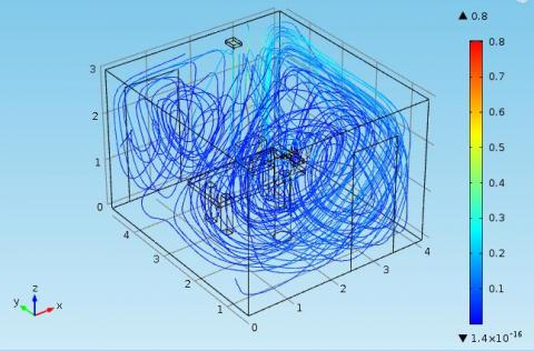
Figure 18. Air flux in winter
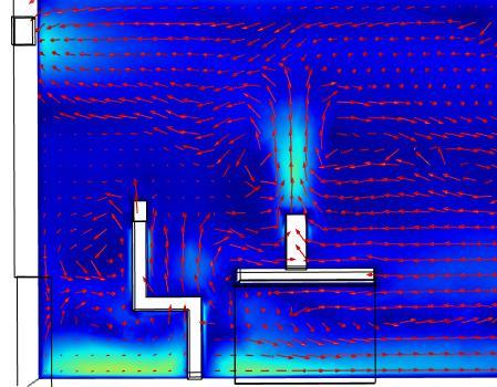
Figure 19. Air flux in summer
The simulations were performed in various scenarios, as summarized in the following table 9.
Table 9. Simulation at various scenarios
|
Parameters |
Seated body |
Seated body and PC off |
Standing body |
Standing body and PC off |
|
|
Temperature [°C] |
Head |
26,864 |
26,693 |
27,223 |
26,972 |
|
|
Feet |
22,41 |
22,119 |
22,234 |
22,019 |
|
Speed [m/s] |
Head |
0,01127 |
0,00311 |
0,02204 |
0,02127 |
|
Feet |
0,13569 |
0,13009 |
0,16345 |
0,16155 |
|
The vertical distribution of the temperature is given in table 10 for the summer and table 11 for the winter.
Table 10. Vertical distribution of the temperature in summer
|
Point |
Temperature [°C] |
|
|
Head |
Feet |
|
|
1 |
19,081 |
16,928 |
|
2 |
19,076 |
16,868 |
|
3 |
19,078 |
16,853 |
|
4 |
19,063 |
16,873 |
|
Mean |
19,075 |
16,88 |
Table 11. Vertical distribution of the air speed in winter
|
Point |
Speed [m/s] |
|
|
Head |
Feet |
|
|
1 |
0,0117 |
0,0062 |
|
2 |
0,0091 |
0,0103 |
|
3 |
0,0101 |
0,0214 |
|
4 |
0,0075 |
0,0259 |
|
Mean |
0,0096 |
0,0159 |
Simulations were carried, but not shown here, in transient condition. From the obtained outputs it’s possible to observe that the displacement system allows to reduce considerably the air flow rate during summer cooling (reduction compared to primary air is around 60%). On the contrary, in winter there is an increase of approximately 12% in the air flow.
A further advantage represented by the displacement systems, compared to an all-air system, concerns the air speed values in correspondence of the occupants; in fact, because of the characteristics of the mixing systems, traditional air systems promote the air at velocity higher than that of the displacement system.
High air speeds could cause considerable discomfort for occupants.
Other simulations with the airflow vent at the other side of the wall are not presented here but give comparable outcomes.
The CFD simulations of air conditioning systems allow to get a lot of information on fluid-dynamic distribution inside the occupied spaces. Simulations for a typical office room showed that displacement systems have higher efficiency and make indoor air quality good. The use of primary air and fan coil systems allows to cover easily the thermal or cooling load and rapidly reach design conditions. External walls (specifically their mass and their transmittance) may play an important role in thermal transients and in HVAC control.
Cp specific heat at constant pressure (J/(kg·K))
F magnitude of buoyancy force (N/m3)
h convective coefficient (W/(m2·K))
k thermal conductivity (W/(m·K))
p pressure (Pa)
u magnitude of speed vector (m/s)
Q metabolic heat (W)
t time (s)
T temperature (K)
η ventilation effectiveness
μ dynamic viscosity (Pa·s)
ρ density (kg/m3)
Subscripts
atm atmospheric
ext external
in Inlet
out outlet
T turbulent
[1] Petrone G., Cammarata L. and Cammarata G., “Bio-effluents tracing in ventilated aircraft cabins,” Proceedings of COMSOL Conference 2009, Milan, Italy.
[2] Petrone G., Cammarata L. and Cammarata G., “A multi-physical simulation on the IAQ in a movie theatre equipped by different ventilating systems,” Building Simulation, vol. 4, no. 21-31, 2011. DOI: 10.1007/s12273-011-0027-6.
[3] Balocco C., Petrone G. and Cammarata G., “Assessing the effects of sliding doors on an operating theatre climate,” Building Simulation, vol. 5, pp. 7383, 2012.
[4] Balocco C., Petrone G. and Cammarata G., “Numerical multi-physical approach for the assessment of coupled heat and moisture transfer combined with people movements in historical buildings,” Building Simulation, vol. 7, pp. 289-303, 2014. DOI 10.1007/s12273-013-0146-3.
[5] Balocco, C., Petrone and G., Cammarata, “Numerical multi-physical approach for the assessment of coupled heat and moisture transfer combined with people movements in historical buildings,” Building Simulation: An International Journal, vol. 7, pp. 289-303.
[6] Balocco, C., Petrone, G., Cammarata, G., Vitali, P. Albertini, R. and Pasquarella, C. I., “Indoor air quality in a real operating theatre under effective use conditions,” J. Biomedical Science and Engineering, vol. 7, pp. 866-883, 2014.
[7] Balocco, C., Petrone, G., Cammarata, G., Vitali, P. Albertini, R. and Pasquarella C.I., “Experimental and numerical investigation on airflow and climate in a real operating theatre under effective use conditions,” International Journal of Ventilation, vol. 13, no. 4, pp. 351-368, 2015.
[8] Balocco C., Petrone G. and Cammarata G., “Thermo-fluid dynamics analysis and air quality for different ventilation patterns in an operating theatre,” International Journal of Heat and Technology, vol. 33, no. 4, pp. 25-32, 2015.
[9] Balocco C., Petrone G. and Cammarata G., “Numerical investigation of different airflow schemes in a real operating theatre,” J. Biomedical Science and Engineering, vol. 87, pp. 73-89, 2015.
[10] EN 15026-2007, Hygrothermal performance of building components and building elements, Assessment of moisture transfer by numerical simulation, Standard, 2007.
[11] Ignat L., Pelletier D. and Ilinca F., “A universal formulation of two equation models for adaptive computation of turbulent flows,” Computer Methods in Applied Mechanics and Engineering, vol. 189, pp. 1119 1139, 2000.
[12] Launder, B. E. and Spalding, D. B., “The numerical computation of turbulent flows,” Computer Methods in Applied Mechanics and Engineering, vol. 3, pp. 269-289, 1974.
[13] Deuflhard, P., “A modified newton method for the solution of ill-conditioned systems of nonlinear equations with application to multiple shooting,” Numerische Mathematik, vol. 22, pp. 289-315, 1974.
[14] Launder B. E., Spalding D. B., “The numerical computation of turbulent flows. Computer methods in applied mechanics and engineering,” Computer Methods in Applied Mechanics and Engineering, 3: 269 −289, 1974.
[15] Zhang L., Chow T. T., Fog K. F., Tsang C. F. and Qiuwang W., “Comparison of performances of displacement and mixing ventilations. Part II: indoor air quality,” International Journal of Refrigeration, vol. 28, pp. 288 −305, 2005.
[16] ANSI/ASHRAE (2004b). Standard 62.1-2004. Ventilation for Acceptable Indoor Air Quality. Atlanta: American Society of Heating, Refrigerating and Air-Conditioning Engineers, Inc.
[17] ASHRAE Standard 62-2001 (2001). Ventilation for Acceptable Indoor Air Quality.
[18] ANSI/ASHRAE (2004a). Standard 55-2204. Thermal Environmental Conditions for Human Occupancy. Atlanta: American Society of Heating, Refrigerating and Air-Conditioning Engineers, Inc.
[19] ANSI ASHRAE Standard 55, Thermal Environmental Conditions for Human Occupancy, ASHRAE Standards Committee, the ASHRAE Board of Directors, and the American National Standards Institute, USA, 2013.
[20] ASHRAE Handbook, Heating, Ventilating, and Air-Conditioning Applications, SI Edition, 21.1–21.23, 2011.
[21] Bauman F., Underfloor Air Distribution (UFAD) Design Guide, American Society of Heating, Refrigerating, and Air Conditioning Engineers Research Project RP-1064, Atlanta, 2003.
[22] Hindmarsh H., Brown A. C., Grant P. N., Lee K. E., Serban S. L., Shumaker R., Woodward D. E., and Woodward C. S., “SUNDIALS: Suite of nonlinear and differential/algebraic equation solvers,” ACM Transactions on Mathematical Software, vol. 31, pp. 363 396, 2005.
[23] UNI EN ISO 7730, “Ergonomics of the thermal environment. Analytical determination and interpretation of thermal comfort using calculation of the PMV and PPD,” 2006.
[24] ISO, Standard 7730, Moderate thermal environments—Determination of the PMV and PPD indices and specification of the conditions for thermal comfort. Geneva: International Organization for Standardization, 1994.