OPEN ACCESS
Basketball game flow and its design can be described as in many others natural systems. The structure, shape and functionality evolve in time and are closely related to performance in several sports. Basketball is a collaboration-opposition sport, thus games present critical points. Non-linear local interactions among players are reflected in the score evolution, the order parameter. Some researchers often presume that scoring in basketball is a random process, meaning memoryless, described using Poisson Model. Scoring cannot be described by a unique distribution. We examined 6130 NBA games and analyzed time intervals between points and scoring dynamic. In the NBA, the most competed games are decided in the last minute, where fouls play a main role (94.02%). Both teams try to keep their advantage solely in order to reach the last minute, where a different game will be played, which can be considered as an example of Red Queen Hypothesis. We also measured the game flow through players real interactions: passes, screens and space creations. Data follow a homogeneous distribution up to a certain value, suggesting that teams resolve the situation with a few steps (diffuse flow). But, if the situation becomes more critical, the dynamics turn into a Power Law Distribution, they modify the game flow spontaneously into a Scale-Free flow (hierarchical flow). These processes take place simultaneously and continuously during game time. Therefore teams would be considered as self-organizing systems.
Basketball, Game Flow Design, Self-Organization, Power Law, NBA.
Sports have proven to be a good field for analyzing dynamic systems, Sports provide a rich laboratory in which to study competitive behavior in a well-defined way [1]; e.g. random walk, complex statistics or extreme events [1, 2], game theory [3] and also in the construction and exploration of models, dynamics of competition [4]; particularly in basketball. In the context of analyzing adaptation, this conceptual linkage can be described by the Constructal Law. Constructal Law states that all systems evolve into the direction to maximize access for all flows through it. Constructal Law is also that systems that keep the capacity for structural adaptation will be favoured enhanced. In other words, flow-maximizing structures need to maintain evolvabilit y [5].
In basketball, most investigations have focused in the classic statistic, based on Poisson Model, Negative Binomial or Extreme Events. And also, statistical models more related to complexity such as Power Laws (PL), q-statistics, etc. [4, 6–8]. A priori, as most of authors point out, scoring in basketball can be considered as a random process, meaning memoryless [1, 4].
Nevertheless, scoring in basketball present some specific features e.g. fouls dynamic (free throws), which comes up from the game. This fact gives to the game a much more complex character, thus the issue of exclusive use of statistical models may be challenged.
For that reason, in the first part of this paper we focused on the consecutive points scored by any of both teams in each game. Therefore a game can be considered as an arrival process; where in a time interval (DT) is scored a number n of field goals. Using the Poisson model as a reference, the complex dynamic will emerge from the edge of this model. Therefore, to understand the underlying Poissonian process, if exists, it is important to define the time interval that we used to determine the rate or speed at which the game is conducted. That is, we determine with what DT we "observe" the game. Hence for a time interval DT a l value is defined as the mean number of events for time interval or l=µ*DT, being µ the number of events per seconds.
The sample analyzed were 5 NBA Regular Seasons (no play-off), a total of 6130 games that we considered enough to be able to analyze short time intervals, minimum DT=2 seconds. We excluded the over-times in order to analyze a homogeneous sample, which contain all kind of games with several competitive realities. The over-times and play-off correspond to different games somehow, which would bias our analysis. Also we examine the possible presence of scale free or PL distributions, a type of ubiquitous behavior in dynamic systems and in the basis of statistical type [9].
The second part of this work deal with the real game flow in a basketball game. A long-standing problem in biological and social sciences is to understand the conditions required for the emergence and maintenance of cooperation in evolving populations [10, 11]. The aim should be cooperation without reciprocity, without selfishness. As Phil Jackson said: to put the "me" in service of the "we” [12]. In fact, collaboration among teammates allows team to compete against other teams. But at the same time confrontation between teams produces a critical situation, which leads to players selection. It can seem simple but it does not. The selection of roster, coaches, staff, etc., by basketball teams is vital (for instance the combination between veterans and rookie players and great head coaches).
In a basketball game, game flow does not remain stable. Teams try to modify their shape and structure in order to enhance their attributes; consequently, actions of players contain information. We assume that teams behave as a whole. Game flow is expressed by real interactions of players. These interactions are Passes, Screens and Space Creations. We consider each possession (each play) as a particular situation; so in a single game there are numerous plays. In consequence, we measured how many manifestations of the system took place in a critical game. Self-organization is patent when a team modifies his structure or game flow (cooperation) spontaneously through local interactions in order to overcome the critical situation. Usually, discussions about functionality are based on team structure, which possesses inherent characteristics. Here are shown a great example of how indeed each model displays different properties and the self-organization is based in the plasticity from a model to other according to an order parameter: Scoring [2].
We study the last game of 2011 Eastern Conference NBA Finals, Chicago Bulls vs. Miami Heat, as sample of a high competed game (score difference remained lower 10 points) which displays a critical profile (de Saá Guerra et al., 2013). We measured for each team the number or Passes, Screens and Space Creations performed per play. Passes represent the clearest example of players interaction. Screens are aimed to neutralize a teammate defender, in order to provide a superiority situation. This point is related whit next. After a screen, or just itself, Space creation happens when a player is occupying a court location and leaves that space to perform a clear out play, or a curl cut play (e.g. the famous UCLA cut).
When a process follows a Poisson distribution, the events must be random and independent. But if the independence is broken, this can lead to Pareto or PL distributions. As Andriani and Mc Kelvey [13, 14] suggest, within competitive systems the PL type distributions can show up under two conditions: when the competitive intensity increases and when the cost of connections or of information transmission decreases. A specific structural design can facilitate the transmission of information much more efficiently, improving the self-organization ability and the recovery capacity of the system against perturbations [15].
A basketball game is a competitive system. During the game time, this competitiveness can fluctuate; hence competitive intensity may be much higher at certain times of the game than others. In the final moments of greatly competed games, one team has a small advantage over the other and tries to keep it the remaining time. The team which does not lead the score will try to wipe out this difference. The issue is that in the final moments of the game, the uncertainty (officials, fatigue, injures, wrong decision, etc.) could be key. Thus, is in these moments when an effective management and make decision are more necessary, the information among all elements of the system and the interrelation between them should flow more easily. The complexity of the game hence, may increase, which in some way be reflected in the number and type of points that are achieved. The struggle to regain the relative advantages in a complex environment, which seems to have some resemblance to a Red Queen's race, has many solutions: keep the possession, forcing shots, make quick fouls, etc. Thus we can expect to emerge avalanche events in the number of points achieved, affecting the tail of the distribution and the probability of power law distributed phenomena increases substantially.
There are several paths to analyze a basketball game from a Poissonian point of view. First at all, we selected different values of DT and the number of points scored in each time interval for both teams in all competitions considered. In Table 1 are shown, for each time interval, the mean values (l), the variance values, the Index of Dispersion (ID) (variance mean ratio) and the ratio between the number of zeros expected by Poisson and the number of real zeros or Index of Zero (I0),) of the entire sample. A linear fit between the first two columns,
l = µ DT+c,
gives us the mean value μ = 0.038 in points scored per second, c = -0.0008 and R2=1.
Table 1. Statistics for the number of baskets (points) in the set of all the games in different time intervals (DT)
|
dT in seconds |
Mean (l) |
Variance |
ID (Var/Mean) |
IO |
|
2 |
0.077 |
0.095 |
1.23 |
0.99 |
|
3 |
0.115 |
0.138 |
1.19 |
0.98 |
|
4 |
0.154 |
0.179 |
1.16 |
0.98 |
|
5 |
0.192 |
0.218 |
1.13 |
0.98 |
|
6 |
0.231 |
0.254 |
1.10 |
0.98 |
|
8 |
0.308 |
0.321 |
1.03 |
0.99 |
|
10 |
0.385 |
0.379 |
0.98 |
1.00 |
|
15 |
0.578 |
0.512 |
0.88 |
1.05 |
|
20 |
0.771 |
0.655 |
0.84 |
1.11 |
|
30 |
1.157 |
0.971 |
0.83 |
1.22 |
|
40 |
1.543 |
1.288 |
0.83 |
1.34 |
|
48 |
1.852 |
1.554 |
0.83 |
1.43 |
|
60 |
2.315 |
1.955 |
0.84 |
1.59 |
|
90 |
3.473 |
2.999 |
0.86 |
1.91 |
Taking into account that the ID value in a Poisson process is 1, we can obsever that the ID values decay linearly up d t = 10 sec., remaining almost constant from dt = 30 sec. The I0 value is almost constant and slightly less than 1 for small values of dt, it is 1 around dt = 10 sec. and then increases linearly. For values D T <8 the variance is greater than average, but as the value of I0 is maintained close to 1, the over-dispersion is due to increase in the tail of the distribution.
The ID values approach to 1 in values around 8-10 seconds, then drops below 1 (sub-dispersion). In this case, the ratio between the number of zeros expected by Poisson and the number of real zeros increases, which means a lower number of zeros respect to Poisson, reflecting that in basketball scoring is not an event as rare as in other sports, with a lower variance and also a lower probability in the tail than the Poisson distribution. We will discuss this deeply later.
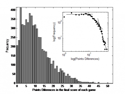
In a recent paper [2], we noted that the final point differences seems to follow several Power Laws (PL). Most of them ended with differences lower than 10-11 points, which were distributed almost uniformly and correspond to the most competed games.
Figure 1. Histogram of final point differences. The upper panel represents the log-log of the histogram. This displays three different PL which points out three different game profiles
The Figure 1 shows the histogram of the final point differences for the entire sample analyzed. The log-log (upper panel) suggests the presence of more than one PL, with two crossovers located around final difference of 11 and 27 points. A total of 3846 games (63%) concluded with a difference between 1 and 11 points, 1854 games (30%) had a difference between 12 and 26 points approximately, and only 7% (431) did so with a difference of 27 or more points. Here we use Power Law only conceptually. We do not mind its exact fit. The appearance of these PL helps us to classify the entire sample in competed games and non-competed games. In the competed zone (0-11 pts.) the PL presents a slope close to 0, the distribution is approximately uniform and the probability of finishing a game by 2 points is the same as 10 points; this is a notable fact. In turn, games finished in zero are relatively scarce in basketball (excluded over times), while finishing by two points difference has a higher probability because the scoring mechanism breaks the symmetry (2 pts or free throws). We defined this kind of games as competed games. It is notable that there are not a number of points that characterize the end of a competitive game, having the same probability between 1 and 11. A typical final score does not exist. From 12 to 27 there is another region where the PL has a negative exponent; there is any superiority of one team over another. These games are more predictable than the previous but still competed. The last case, point difference higher than 27, are games with a clear dominance of a team. These games (7%) are few compared to the rest, for that reason we consider games finished by 0-11 points as competed games, and with point differences higher than 11 as non-competed games.
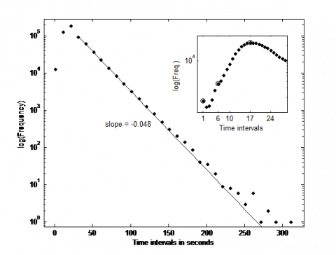
In [1, 2, 4] are shown the distribution of time intervals between points (dt), that in a Poisson process would be an exponential distribution. In Figure 2, we represent the same distribution in a semi-log-plot, but with an important difference. In the upper panel we highlight the detail for dt < 30 seconds. Note that beyond 26 seconds the data follows an exponential distribution (solid line in figure and µ value) with µ = 0.048 slightly higher than that obtained before by linear fit. We noted [2] that after 100 seconds, the probability of remain without scoring is greater than that provided by the exponential distribution, this seems to be a memory effect that exponential distribution does not have (memorylessness). I.e. if the game gets complicated and neither of teams scores after a critical time, the probability of not scoring in the next few seconds seems to increase, which occurs in the first minutes of each quarter and especially in the fourth quarter.
Figure 2. Semi-log plot of point time intervals frequency. Apparently, there are three different behaviors. The data follow a distribution with a maximum (peak) around 20 seconds. Beyond 30 seconds follows an exponential distribution. The upper panel represents a detail for the first 30 seconds
Table 2 shows the percentage of points with time difference between them dt = 1, 2..., 8 seconds; and the minute in which take place. "Others" represents the values for remaining minutes in the game. The lower part shows the result for the same time differences but for each type of points (1, 2 or 3).
Table 2. Percentage of points for different dt. And for 1pt, 2pt and 3 pt
|
Minute of the game |
dt=1 |
dt=2 |
dt=3 |
dt=4 |
dt=5 |
dt=6 |
dt=7 |
dt=8 |
|
|
11-12 |
1.52 |
4.38 |
5.45 |
6.28 |
5.38 |
5.13 |
5.12 |
4.26 |
|
|
23-24 |
3.45 |
5.99 |
7.92 |
7.98 |
7.92 |
6.44 |
6.27 |
5.56 |
|
|
35-36 |
2.98 |
3.76 |
5.96 |
6.50 |
6.16 |
4.15 |
4.88 |
4.49 |
|
|
46-47 |
3.39 |
4.61 |
6.40 |
6.61 |
6.27 |
5.48 |
5.89 |
5.30 |
|
|
47-48 |
69.68 |
57.07 |
45.64 |
40.53 |
32.36 |
22.80 |
19.96 |
12.95 |
|
|
Others |
18.98 |
24.19 |
28.63 |
32.10 |
41.91 |
56.00 |
57.89 |
67.45 |
|
|
1 |
89.18 |
69.39 |
54.76 |
45.54 |
44.78 |
39.97 |
39.62 |
37.49 |
|
|
2 |
8.01 |
20.84 |
33.09 |
42.13 |
44.26 |
48.98 |
48.65 |
50.27 |
|
|
3 |
2.81 |
9.08 |
12.15 |
12.33 |
10.96 |
11.06 |
11.73 |
12.24 |
|
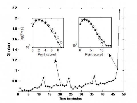
To better understand the limitations of the Poisson Model, let´s assume that every minute in a basketball game behaves as a Poisson process. Consequently, we could calculate the probability of number of points scored in the first minute for the entire games, in the second, in the third and so on. Every minute is considered an independent Poisson process. The following Figure (Figure 4) displays the ID every single minute. In general, the variance values are lower than the mean values, a sub-disperse case, and hence is more predictable than the pure Poisson process. The ID increases along with game evolution, pointing out more randomness. Particularity, the last minutes of the three first quarters approach to 1; as well the minute 47, which presents value 1. The upper panels illustrate the frequency of the number of scored points in a semi-log plot (dotted solid line) for two cases: minute 20 and minute 47. We both compared to Poisson distribution (dash line (o)). In the first case the variance is lower than predicted by Poisson. The minute 47 behaves similar to final minutes in previous quarters and matches the Poisson distribution but for some tail values, with a low weight in the total distribution. The case of minute 48 is totally different from the rest of the game.
Figure 4. Index of Dispersion of the point scored by minute
We can observe that the trend of the values is to rise over time. Only at the end of each quarter there are a significantly increase, closer to 1, but only at the minute 47 reach the value 1 (pure Poisson). The minute 48 is completely out the range of the rest of the game, reaching values higher than 1. The behavior of this minute is very complex. The two upper panels represent the point frequencies semi-log plot (dotted solid line) and Poisson distribution (dash line (o)) for the minute 20 (left) and the minute 47 (right).
In order to a better understanding, we have selected some cases with representative Index of Dispersion. We analyze two minutes intermediate 6 and 32, a quarter final minute 36 and the minute 47, with Index of Dispersion values 0.63, 0.75, 0.90 and 1.02 respectively.
Figure 5. Histograms of the point scored in the minutes 6, 32, 36 and 47, corresponding to Index of Dispersion values 0.63, 0.75, 0.90 and 1.02
The solid line represents the Poisson theoretical distribution. The two upper cases show under-dispersion, whereas the lower cases present an Index of Dispersion close to 1, with a Poissonian behavior.
In the two upper Figures, we observe that do not fit well to the Poisson distribution, ID < 1, and data are clustered around mean value, with less zeros and a lower probability values in the tail than Poisson, characterizing an under-dispersed Poisson distribution. In general, are more predictable than a pure Poisson process.On the other hand, in the two cases below, the Poisson distribution fits better (Index of Dispersion 0.90 and 1.02). Note that the number of zeros matches better and decays as Poisson. The minute 47 represents the most unpredictable moment of the game, except the last minute, which will be treated separately because the nature of the distribution is different. This seems to be an indicator of the risk assumed by teams. Teams tend to risk more at these times, and defensive intensity increases (more fouls) which indicates greater likelihood of failures, more zeros than in previous times or greater number of points (longer tail), meaning great randomness and explain its proximity to the Poisson distribution. In the cases with less risk (two upper subplots), the game seems more predictable and the number of failures is lower; which would justify the least number of zeros and the shorter tail.
In the last minute the variance is significantly higher than the mean, indicating an over-disperse case which can be modeled by a Negative Binomial Distribution. The Figure 6 shows the scored points histogram and the Negative Binomial Fit (parameters 3.86 +/- 0.27; 0.48 +/- 0.02). The source of this behavior could be the clusterization of scored points and focused in some specific games where the number of scored points increases. We carried out a scaling analysis by a log-log plot (upper panel) which reveals that the data can be fitted by a PL as well, with a crossover around 9 points, and it is shown only for qualitative purpose. Hence, we can deduce that there are three situations: less than 4 points, between 4 and 8 points and more than 8 points in the last minute. Even it its possible reaching 20 points or more in the last minute, which points out the complexity of the game and importance of as is shown in Table 2.
Figure 6. Histogram of point scored in the last minute of the game
The solid line represents negative binomial distribution fit. Note that the values are better fitted at the tail of the distribution. For further analysis, we carried out a log-log plot, in the upper panel, which displays two Power Laws with a crossover (straights lines). The dashed line in the upper panel represents the negative binomial fit.
As we just have seen, basketball is not a random game. The reality is much more complex that we might think in advance, where the game flow does not remain stable or predictable. The second part of this work tries to figure out the basketball team reality in a real basketball game. We analyzed a competed game and measured the game flow through interactions of players.
The Figure 7 represent the histogram of the number of Passes, Screens and Space Creations. The x-axis represents the number of events in a single play. The y-axis represents the number of plays with the number of events happened. Regarding Passes, Chicago (right column) reaches up to eight passes per play, whereas Miami (left column) only achieves five passes maximum. The absolute number of Miami plays is lower than Chicago. The scaling analysis (upper panels) reveals that the distributions decay as a Power Laws $P(k) \approx k^{-\gamma}$. The presence of this truncated Power Laws points out different dynamics regarding passing. Note that the cut for Chicago is located in four passes, but for Miami is located around three.
Regarding screens, the histogram of Chicago decays; while that the predominant situation in Miami is one single screen. Moreover, sometimes Chicago performs plays with up to five screens; one more than Miami. When we carried out a log-log plot, note a cut in two screens for Chicago and two cuts in Miami. This fact gives us a lot of information about the Miami game style. The core situation for Miami is one screen mainly, or no screens. Chicago and Miami display different profiles regarding space creations. Chicago seems to behave a homogeneous region from zero to two space creations, and the values drops from this point. In contrast, Miami shows a predominance of one space creation even though zero space creations values are similar. The log-log plot reveals two different areas in Chicago and three in Miami.
Figure 7. Histograms of Chicago (right column) and Miami (left column) passes, screens and space creations respectively.
X-axis represents the number of events in a single play and the y-axis represents the number of plays with that number of events. The log-log plots (subplots) show several tipping points in the sample analyzed. This fact reveals different realities. The tails of the distributions follow an approximate Power Law to Chicago with exponent gChipasses » 3.8; gChiscreens1 » 2.2; gChiscreens2 » 7.2; gChispaces » 1.7; and to Miami with exponent gMiapasses » 5.8; gMiascreens1 » 1.2; gMiascreens2 » 4.2; gMiaspaces1 » 0.6; gMiaspaces2 » 3.2.
The conclusion than can be draw is if players are able to resolve the situation despite the opposition of rival team with a few interactions (number of interactions with a homogeneous probability, the game flow can be considered as diffuse, in the sense that only with a few steps, they resolve the situation. Game flow preserves their inherent structure despite a substantial number of attacks or disturbances [16]. This can be interpreted as that, indeed, when a team is in a stable situation, suffers constantly attacks by the other team, but maintains its structure throughout the game.
But when team exceeds the first tipping point, the distribution decays as a Power Law with a degree distribution to Chicago: gChipasses » 3.8; gChiscreens1 » 2.2; gChiscreens2 » 7.2; gChispaces » 1.7. and to Miami gMiapasses » 5.8; gMiascreens1 » 1.2; gMiascreens2 » 4.2; gMiaspaces1 » 0.6; gMiaspaces2 » 3.2. The Power Laws indicate that now they behave as a Scale-Free flow meaning that some players absorb more game flow than the others. Therefore, game flow is focused in some players. The team becomes from a diffuse flow to a concentrated flow, a hierarchical flow.
This does not necessarily means that the player who focuses the game is the player who carries out all shoots. It also can be a game distributor or game creator. Or just an emergency from the game caused by time (time runs out) or specific game situation. Given the high degree of randomness that exists in most games with an 11-point difference or lower, we could suppose that the majority of games have a high degree of uncertainty. Therefore it is very difficult to know in advance how players will behave. But we observed that there are patterns that emerge spontaneously in response to needs or survival tactics in the game. In fact, the team success (attack or defense) depends on those action sequences.
In sort, a basketball team can be considered as a good example of self-organization. Defenders collaborate in order to hamper the flow of the attackers. But at the same time attacking players try to overcome this opposition through their skills as team. It is a collaboration-opposition sport. The multiple local interactions among teammates and opponents (mainly non-linear type) influence on each other and confer the game a critical profile. All these processes take place simultaneously and continuously during game time. In fact, that is what make sport attractive to fans and media (and enables to survive and improve), the ability of teams of arising out new behaviors.
1. A. Gabel and S. Redner, J. Quant, Anal. Sports, 8, (2012).
2. Y. de Saá Guerra, J.M. Martín Gonzalez, S.S. Montesdeoca, D. Rodriguez Ruiz, N. Arjo-nilla López, and J. M. García Manso, J. Syst. Sci. Complex, 26, 94 (2013).
3. B. Skinner, J. Quant, Anal. Sports, 6, (2010).
4. S. Merritt and A. Clauset, EPJ Data Sci., 3, 4 (2014).
5. A. Bejan and S. Lorente, J. Appl. Phys., 100, 041301 (2006).
6. A. Heuer, C. Mueller, and O. Rubner, arXiv: 1002.0797 (2010).
7. L. Malacarne and R. Mendes, Phys. Stat. Mech., Its Appl., 286, 391 (2000).
8. H. V. Ribeiro, R. S. Mendes, L. C. Malacarne, S. P. Jr, and P. A. Santoro, Eur. Phys. J., B 75, 8 (2010).
9. M. Newman, Contemp. Phys., 46, 323 (2005).
10. R.L. Riolo, M.D. Cohen, and R. Axelrod, Nature, 414, 441 (2001).
11. R. Guimera, B. Uzzi, J. Spiro, and L.A.N. Amaral, Science, 308, 697 (2005).
12. P. Jackson and H. Delehanty, Sacred Hoops: Spiritual Lessons of a Hardwood Warrior, Hyperion Books, 2006).
13. P. Andriani and B. McKelvey, J. Int. Bus. Stud., 38, 1212 (2007).
14. P. Andriani and B. McKelvey, Organ. Sci., 20, 1053 (2009).
15. S. H. Strogatz, Nature, 410, 268 (2001).
16. B. Uzzi, L. A. Amaral, and F. Reed-tsochas, Small-World Networks and Management Science Research: A Review (2007).