OPEN ACCESS
Finite element simulation is performed visualizing heat flow through heatlines for a free convection flow and heat transfer in an air-filled prismatic enclosure. This configuration has applications in collecting solar energy in attic spaces of greenhouses and buildings having pitched roofs. The top inclined walls of the enclosure are considered at constant low temperature, two vertical walls are adiabatic whereas the bottom wall is heated isothermally as well as non-isothermally. The Galerkin weighted residual finite element method is used to solve the governing non-linear partial differential equations. The simulated results are displayed through streamlines, isotherms and heatlines to examine the effects of buoyancy on the flow and thermal fields. The Rayleigh number’s effects on average temperature and velocity fields are also calculated and displayed graphically. The results indicate that for a uniformly heated bottom wall both the average temperature and the average velocity in the cavity are higher compared to the non-uniformly heated bottom wall. Furthermore, heatlines were observed to predict the energy transfer better than those of the isothermal lines.
Heatline, Natural convection, Heat transfer, Prismatic enclosure, Finite element method.
Heat transfer through buoyancy induced flow is an important engineering phenomenon which has direct applications in solar thermal collectors, cooling of electronic devices, nuclear reactors, controlling fire, measuring air movement in attics and greenhouses. Experimental and/or numerical studies generally concern square or triangular shaped enclosures. However, free convection flow and heat transfer in a prismatic enclosure is frequently found in attic areas of domestic buildings. Walid and Ahmed [1] studied buoyancy induced heat transfer and fluid flow inside a prismatic cavity. Their results revealed that the cavity's aspect ratio has a significant influence on the temperature and flow fields. Walid et al. [2] performed numerical analysis of natural convection in a prismatic enclosure. Their results indicated that heat transfer rate increases with increasing the Rayleigh number and decreases with increasing aspect ratio. Recently, Yaseen [3] studied numerically the steady natural convection flow in a prismatic enclosure with strip heater on the bottom wall. From his study it is seen that the Rayleigh number, the location of strip heaters and the number of heaters remarkably affected the flow and thermal fields.
The streamlines adequately depict the fluid flow but isotherms represent only temperature distribution that may not be sufficient to visualize the transport of heat. The technique of heatline is one of the best ways of visualizing the heat recovery system or true path of heat transfer due to convection. The concept of heatline was developed (see Kimura and Bejan [4], Bejan [5]) to visualize the conductive along with convective heat transports. Heatlines typically represent the heat functions which intrinsically satisfy the energy equation while a stream function satisfies the mass conservation equation. Heatlines are related to the Nusselt number depending on the dimensionless form of transformations. Bello-Ochende [6] investigated thermal convection in a square cavity considering Poisson type heat function. Morega and Bejan [7] visualized heatlines for a convective laminar boundary layer flow on a flat plate having zero flux or uniform temperature. On the other hand, Zhao et al. [8] explored numerically the applications of heatlines, masslines and streamlines for conjugate heat and mass transfer. They have established that heatlines and masslines are effective tools discussing the heat and mass transfer mechanisms. They further reported that the results visualized by heatlines, masslines and streamlines directly exhibit the nature of the fluid; the heat and mass transports through solid bodies and the diffusive walls of the cavity. The processes of unification of heatline, massline and stream line to visualize the two-dimensional transport phenomena are described by Costa [9]. Costa [10] further reviewed the concepts of Bejan’s heatlines and masslines for convection visualization. To visualize the path of heat flow through heat function in a buoyancy driven turbulent flow over a heated vertical flat plate was introduced by Dash [11]. Zhao et al. [12] investigated double-diffusive nantual convection in an enclosure with localized heating and salting from below. They have demonstrated heatlines, masslines and streamlines to visualize the heat and fluid flows. The heatline applications may further involve conjugate natural convection or heat conduction (see Liu et al. [13], Zhao et al. [14]), double-diffusive convection in a porous enclosure (see Zhao et al. [15]), and forced convection in a porous media (see Morega and Bejan [16]). However, a comprehensive analysis on heat flow during natural convection in a prismatic enclosure heated from below with the heatline approach has not studied yet. Thus, energy flow throgh heatlines is essential to study.
Motivated from the above-stated studies, we analyze the heat transfer in a prismatic enclosure in order to visualize the heat flow and to find an efficient way of transferring heat in the enclosure. This study may have applications to visualize heat transfer in a roof-type solar still and various other engineering structures. The governing equations for heat and fluid flow, Poisson equations for stream function and heat function are solved using a finite element method. The jump discontinuity in Dirichlet type wall boundary conditions for temperature at corner points correspond to computational singularities. We therefore considered the average temperature of the two walls at the corner point and maintain the adjacent grid nodes at the respective wall temperatures.
Consider a two-dimensional viscous, incompressible, laminar, natural convection flow in a prismatic enclosure filled with air. See Figure 1 for schematic diagram, geometrical details and associated boundary conditions. The horizontal bottom wall is heated isothermally as well as non-isothermally while the inclined walls are maintained at a constant lower temperature and the vertical walls are insulated. Under Boussinesq approximation the governing equations for steady natural convection flow can be written as;
$\frac{\partial u}{\partial x}+\frac{\partial v}{\partial y}=0$(1)
$u \frac{\partial u}{\partial x}+v \frac{\partial u}{\partial y}=-\frac{1}{\rho} \frac{\partial p}{\partial x}+v\left(\frac{\partial^{2} u}{\partial x^{2}}+\frac{\partial^{2} u}{\partial y^{2}}\right)$(2)
$u \frac{\partial v}{\partial x}+v \frac{\partial v}{\partial y}=-\frac{1}{\rho} \frac{\partial p}{\partial y}+v\left(\frac{\partial^{2} v}{\partial x^{2}}+\frac{\partial^{2} v}{\partial y^{2}}\right)+g \beta\left(T-T_{c}\right)$(3)
$u \frac{\partial T}{\partial x}+v \frac{\partial T}{\partial y}=\alpha\left(\frac{\partial^{2} T}{\partial x^{2}}+\frac{\partial^{2} T}{\partial y^{2}}\right)$(4)
The boundary conditions for the above stated model are as follows:
At the bottom wall:
$T=T_{h}$ or $T=T_{c}+\left(T_{h}-T_{c}\right)\left(1-\frac{x}{L}\right)$(5a)
At the top inclined walls:
$T=T_{c}$(5b)
At the vertical walls:
$\frac{\partial T}{\partial x}=0$(5c)
At all solid boundaries:
$u=v=0$(5d)
where the variables and the related quantities have been defined in the nomenclature.
Figure 1. Schematic view of the physical model with boundary conditions
2.1 Dimensional analysis
Dimensional analysis is one of the most important mathematical tools in the study of fluid mechanics. To describe several transport mechanisms in fluid dynamics, it is meaningful to make the governing equations into non-dimensional form. Advantages of non-dimensionalization process can be listed as follows: (i) non-dimensionalization gives freedom to analyze any system irrespective of their material properties, (ii) one can easily understand the controlling flow parameters of the system, (iii) make a generalization of the size and shape of the geometry, and (iv) before doing experiment one can get insight of the physical problem. These aims can be achieved through the appropriate choice of scales. As a scale of distance, we choose the length of the cavity of the region under consideration measured along the $x$-axis.
Thus, in order to reduce the governing equations (1)-(4) along with boundary conditions (5) dimensionless, we incorporate the following transformation of variables:
$X=\frac{x}{L}, Y=\frac{y}{L}, U=\frac{u L}{\alpha}, V=\frac{v L}{\alpha}, P=\frac{p L^{2}}{\rho \alpha^{2}}$
$\theta=\frac{T-T_{c}}{T_{h}-T_{c}}, \operatorname{Pr}=\frac{v}{\alpha}, R a=\frac{g \beta\left(T_{h}-T_{c}\right) L^{3}}{v \alpha}$$\}$(6)
Introducing the relation (6) into equations (1)-(4), the governing dimensional equations can be written in the following dimensionless form:
$\frac{\partial U}{\partial X}+\frac{\partial V}{\partial Y}=0$(7)
$U \frac{\partial U}{\partial X}+V \frac{\partial U}{\partial Y}=-\frac{\partial P}{\partial X}+\operatorname{Pr}\left(\frac{\partial^{2} U}{\partial X^{2}}+\frac{\partial^{2} U}{\partial Y^{2}}\right)$(8)
$U \frac{\partial V}{\partial X}+V \frac{\partial V}{\partial Y}=-\frac{\partial P}{\partial Y}+\operatorname{Pr}\left(\frac{\partial^{2} V}{\partial X^{2}}+\frac{\partial^{2} V}{\partial Y^{2}}\right)+\operatorname{RaPr} \theta$(9)
$U \frac{\partial \theta}{\partial X}+V \frac{\partial \theta}{\partial Y}=\left(\frac{\partial^{2} \theta}{\partial X^{2}}+\frac{\partial^{2} \theta}{\partial Y^{2}}\right)$(10)
The dimensionless forms of the boundary conditions are as follows:
At the bottom wall:
$\theta=1$ or $\theta=1-X$ (11a)
At the top inclined walls:
$\theta=0$(11b)
At the vertical walls:
$\frac{\partial \theta}{\partial X}=0$(11c)
At all solid boundaries:
$U=V=0$(11d)
The fluid motion is displayed using the stream function $\psi$ which is obtained from the velocity components $U$ and $V$. The stream function $\psi$ and the velocity components for a two-dimensional flows are related by:
$U=\frac{\partial \psi}{\partial Y}$ and $V=-\frac{\partial \psi}{\partial X}$(12)
which give a single equation
$\frac{\partial^{2} \psi}{\partial X^{2}}+\frac{\partial^{2} \psi}{\partial Y^{2}}=\frac{\partial U}{\partial Y}-\frac{\partial V}{\partial X}$(13)
A positive sign of $\psi$ denotes anti-clockwise circulation whereas the negative sign represents clock-wise circulation.
Similarly, a heat function $(\Pi)$ can be defined from the conductive heat fluxes$\left(-\frac{\partial \theta}{\partial X},-\frac{\partial \theta}{\partial Y}\right)$ as well as convective heat fluxes $(U \theta, V \theta)$. The heat function satisfies the steady energy equation (10) such that
$\frac{\partial \Pi}{\partial Y}=U \theta-\frac{\partial \theta}{\partial X} \quad$ and $\quad \frac{\partial \Pi}{\partial X}=-V \theta+\frac{\partial \theta}{\partial Y}$(14)
Equation (14) gives a single equation as follows
$\frac{\partial^{2} \Pi}{\partial X^{2}}+\frac{\partial^{2} \Pi}{\partial Y^{2}}=\frac{\partial}{\partial Y}(U \theta)-\frac{\partial}{\partial X}(V \theta)$(15)
The average Nusselt number, average temperature and average velocity can be expressed respectively as
$N u=-\frac{1}{S} \int_{0}^{S} \sqrt{\left(\frac{\partial \theta}{\partial X}\right)^{2}+\left(\frac{\partial \theta}{\partial Y}\right)^{2}} d S$(16)
$\theta_{a v}=\int \theta d \overline{V} / \overline{V}$ and $V_{a v}=\int V d \overline{V} / \overline{V}$(17)
where $S$ is the dimensionless length of the surface and $\overline{V}$ is the volume to be accounted.
Finite element method (FEM) is a very powerful numerical technique that can be applied for solving the ordinary as well as partial differential equations related to science and engineering problems. The basic idea of this method is dividing the whole domain into finite number of smaller ones called finite elements. This method is so good in modern engineering analysis and can be used for solving integral equations including fluid mechanics, heat transfer, chemical processing, electrical systems, and many other fields. Thus, the equations (7)-(10) and the boundary conditions (11) are solved numerically by using Galerkin weighted residual finite element method. The details of this method can be found in the works of Zienkiewicz and Taylor [17], Rahman et al. [18-19], Uddin [20], Triki and Hadj-Taieb [21]. In FEM the discretized finite element meshes are composed of non-uniform triangular elements. To develop finite element equations we used six node triangular elements. All of these six nodes are associated with velocities and temperature whereas the corner nodes are associated with pressure only. Thus, a lower order polynomial is required for evaluating pressure which satisfied through the continuity equation. Then Galerkin weighted residual technique transformed the governing nonlinear partial differential equations into a system of integral equations. A Gauss's quadrature method is applied to perform the integration involved in each term of these equations. The obtained nonlinear algebraic equations are modified by imposing the boundary conditions. To solve the set of global nonlinear algebraic equations in the form of matrix, the Newton-Raphson iteration technique has been adapted through partial differential equation solver with MATLAB interface. The convergence criterion of the numerical solution along with error estimation has been set to $\left|\Phi^{m+1}-\Phi^{m}\right| \leq 10^{-5}$ where $\Phi$ is the general dependent variable $(U, V, \theta)$ and $m$ is the number of iteration.
4.1 Mesh generation
In FEM the generation of mesh is a technique to subdivide a domain into a set of sub-domains; called finite elements. The discrete locations are defined by the numerical grid at which the variables are to be calculated. It is basically a discrete representation of the geometric domain on which the problems need to be solved. Proper meshing of a complicated geometry makes FEM a powerful technique solving the boundary value problems occurring in a range of engineering and technological applications. Figure 2 displays mesh configuration of the prismatic domain having triangular finite elements.
Figure 2. Finite element mesh of prismatic domain
4.2 Code validation
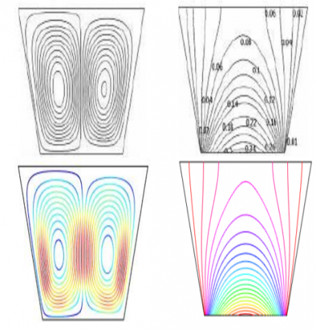
Figure 3. Comparison of streamlines and isotherms with Uddin and Saha [22] (top row) with the present results (bottom row) for their ѱ = 00, $\phi$= 150 and Pr = 0.70 case
To verify the accuracy of the present numerical code, we have compared our results with Uddin and Saha [22] considering $R a=10^{3}, \phi=15^{\circ}, \psi=0^{\circ}$ and $\operatorname{Pr}=0.70$. Figure 3 shows the comparison of the results interms of streamlines and isotherms obtained by our code with those of Uddin and Saha [22]. The results show an excellent agreement and boosts the confidence in using the present umerical code.
Numerical simulations have been done using FEM to analyze natural convective heat transfer and fluid flow within a prismatic enclosure visualizing heatlines. In the next subsections, we will discuss the effects of the model parameters such as the Rayleigh and Prandtl numbers on the flow and heat transfer characteristics with the help of isotherms and streamline patterns. In addition, average temperature and average velocity in the cavity have been calculated for different pertinent parameters.
5.1 Case-I: Linearly heated bottom wall
5.1.1 Effect of Rayleigh number on flow and thermal fields
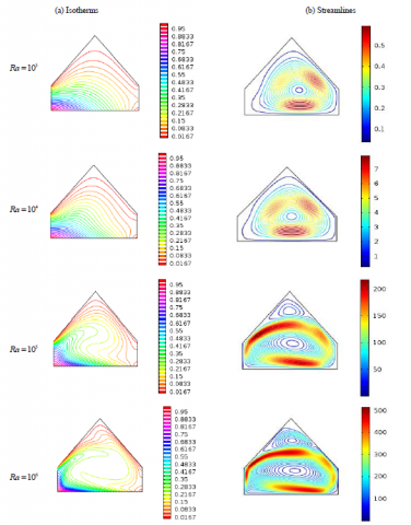
The influence of Rayleigh number Ra (103-106) on isotherms for linearly bottom heated wall at $\operatorname{Pr}=0.7$ has been depicted in Fig. 4(a). The isotherms pattern indicate that at lower $R a=10^{3}-10^{4}$, convection is weaker inside the cavity since they are almost parallel to each other near the heated wall of the cavity. When Rayleigh number increases the convection inside the cavity also increases as a consequence the isotherms become more and more distorted near the middle plane of the cavity forming a pattern like mushroom. This particular pattern suggests that heat energy is flowing into the fluid inside the cavity from bottom heated wall. A higher value of Ra causes higher temperature gradient and thus the isothermal lines move from hot wall to the cold walls.
Figure 4(b) shows the patterns of streamlines for $R a=10^{3}, 10^{4}, 10^{5}, 10^{6}$ from top to bottom respectively. The temperature of the bottom wall is higher than the temperature of the top inclined walls as a result the density of the fluid near the heated bottom wall diminishes compared to the density of the fluid adjacent to the top inclined walls. This results in a clockwise rotation of the fluid inside the cavity as can be seen from these figures. For lower values of Rayleigh numbers ($10^{3}$ and $10^{4}$), the effect of convection is less pronounced and hence, the inertia forces do not make significant contribution to the heat transfer mechanism inside the cavity. An increase in Rayleigh number induces the buoyancy force, resulting a strong circulation of the fluid inside the cavity. A clockwise rotating small vortex is also formed near the upper corner of the cavity.
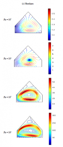
Figure 4(c) illustrates the distributions of heatlines for different values of Rayleigh number when the bottom wall is linearly heated. The heat flow within the enclosure is displayed using the heat function obtained from conductive heat fluxes $\left(-\frac{\partial \theta}{\partial X},-\frac{\partial \theta}{\partial Y}\right)$ as well as convective heat fluxes $(U \theta, V \theta)$. Heatlines arise from hot regimes and end on cold regimes illustrating the path of the heat flow. From this figure, we notice that for low Rayleigh number the heat lines distribute uniformly following clockwise and anticlockwise rotations from the heated wall to the colder wall. In this case, the intensity of the flow is very low and heat transfer occurs mainly due to conduction. We noticed that heat leaves the hot
wall and reseaches the cold wall in an almost uniform way. However, for a high Rayleigh number, the flow intensity is observed significantly. It is also observed that the heat transfer is more intense at the lower heated wall, and relatively colder at the right upper region of the enclosure. In this case, the heat lines are the adequate tools for the visualization and analysis of heat transfer process from hotter wall to the colder wall. As the Rayleigh number increases the heat flows almost look like similar to the streamlines and there is a formation of small vortex near the upper corner of the inclined walls.
Figure 4 (a)-(b). Effects of Rayleigh number Ra on (a) Isotherms and (b) Streamlines for linearly heated bottom wall
Figure 4 (c). Effects of Rayleigh number Ra on (c) Heatlines for linearly heated bottom wall.
Figure 5 (b)-(c). Effects of Rayleigh number Ra on (b) Streamlines and (c) Heatlines for uniformly heated bottom wall
5.2 Case-II: Uniformly heated bottom wall
5.2.1 Effect of Rayleigh number on flow and thermal fields
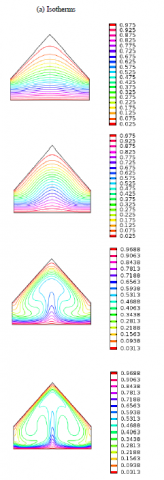
The influences of Rayleigh number $R a=10^{3}-10^{6}$ at $\mathrm{Pr}=0.7$ on the isotherms, streamlines and heatlines for uniformly heated bottom wall case have been shown in Figs. 5(a)-(c) respectively. Isotherm contours detect the effectiveness of heat transfer in a fluid and determine the dictating modes of heat transfer-whether it is conductive or convective. At lower values of Rayleigh number $5(a)-(c)$, the isotherms became almost parallel to the bottom horizontal wall. The density of isotherms is less at the middle of the enclosure, which indicates relatively weaker convective heat transfer for this case. For relatively higher values of $R a$ the isotherms dispersed throughout the enclosure and it increases inside the enclosure. Figure 5(a) confirms the dominance of conduction heat transfer since the isotherms are uniformly distributed. When the Rayleigh number is increased the isotherms become more distorted due to the stronger buoyancy (convection) effects. Figs. 5(a) further depicts that in the middle of the prismatic cavity the isotherms become an inverted mushroom shape which indicate that convection mode of heat transfer is dominant in the region of $R a=10^{5}$ and $R a=10^{6}$. Thus higher $R a$ facilitates convective heat transfer mechanisms.
The streamlines corresponding to uniformly heated bottom wall are displayed in Fig. 5(b). The denisty of the hot fluid near the bottom of the enclosure is lower than the denisty of the cold fluid near the inclined walls. Thus, the less denser fluid near the center of the bottom wall moves upward while the relatively heavy fluid near the cold inclined walls moves downward along the cold walls. The less denser fluid loses energy when moves downward and consiquently forces the thermal boundary layer to separate along the inclined walls. The heavy fluid then enters the thermal boundary layer near the bottom wall and completes the re-circulation pattern. Figure 5(b) shows that for a uniformly heated bottom wall two counter rotating vortices arise inside the enclosure whose eyes are located near the center of each half of the cross-section. This figure also reveals that an increased Rayleigh number intensifies the intensity of the buoyancy driven circulations inside the cavity. The heatlines are drawn based on the isothermal boundary conditions. Figure 5(c) shows that heatlines are smooth and nearly parallel to the vertical lines indicates transport of heat is due to conduction. When the Rayleigh number increased to $R a=10^{6}$, the density of the heatlines near the heated wall also increased and deformation in heatlines became much clear. This leads to higher convective heat transport from the heated walls. In addition, there creates two small vortices at higher Ra, which is consistent with the stream function patterns.
5.3 Average Nusselt number
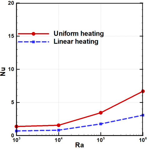
The distributions of the average Nusselt number versus Rayleigh number at the heated bottom wall and cold inclined walls for linearly as well as uniformly heated thermal boundary conditions are presented in Figs. 6(a)-(b), respectively. From these figures we observe that the average Nusselt number increases when the Rayleigh number increases which is utilized to represent the overall heat transfer rate within the flow domain. It is also seen that average Nusselt number increases slowly upto $R a=10^{4}$ and beyond this $R a$ they rise rapidly for both cases. The highest heat transfer rate is observed for a uniformly heated bottom wall case.
(a)
(b)
Figure 6. Average Nusselt number (Nu) at (a) heated bottom wall and (b) cold inclined walls
5.4 Average temperature and average velocity
Figure 7(a) demonstrates the distribution of average temperature versus the Rayleigh number for linearly as well as uniformly heated thermal conditions. We notice that the average temperature rises for increasing the Rayleigh number irrespective of the types of thermal boundary conditions. But highest average temperature is observed when the bottom wall is uniformly heated.
The average velocity within the domain is depicted in Fig. 7(b). In this figure, we see that the average velocities are almost linear upto $R a=10^{4}$ and beyond this region they rise rapidly for both cases. We further observe that the average velocity is higher when the bottom wall is uniformly heated.
Figure 7. Average (a) temperature (Ɵav) and (b) velocity (Vav) in the cavity
In this research we conducted a numerical study to investigate steady natural convective heat transfer and fluid flow inside a prismatic cavity via heatline analysis. Galerkin weighted residual finite element method is applied to obtain smooth solutions for streamlines, isotherms and heatlines. Based on the numerical results, the major findings are listed below:
M. M. Rahman is grateful to The Research Council (TRC) of Oman for funding under the Open Research Grant Program: ORG/SQU/CBS/14/007 and College of Science, Sultan Qaboos University for the grant IG/SCI/DOMS/16/15. M. S. Alam is grateful to TRC for a Postdoctoral Fellowship.
|
$g$ |
acceleration due to gravity |
|
$L$ |
length of the base and height of the cavity |
|
$N u$ |
average Nusselt number |
|
$p$ |
dimensional fluid pressure |
|
$p$ |
dimensionless fluid pressure |
|
$\mathrm{Pr}$ |
Prandtl number |
|
$R a$ |
Rayleigh number |
|
$T$ |
dimensional temperature |
|
$u, v$ |
dimensional velocity components |
|
$U, V$ |
dimensionless velocity components |
|
$W$ |
height of the vertical walls of the cavity |
|
$x, y$ |
dimensional coordinates |
|
$X, Y$ |
dimensionless coordinates |
|
$\alpha$ |
thermal diffusivity |
|
$\beta$ |
coefficient of thermal expansion |
|
$v$ |
kinematic viscosity |
|
$\rho$ |
density |
|
$\theta$ |
dimensionless temperature |
|
$\psi$ |
stream function |
|
$\Pi$ |
heat function |
[1] A. Walid and O. Ahmed, “Buoyancy induced heat transfer and fluid flow inside a prismatic cavity,” J. Appl. Fluid Mech., vol. 3, no. 2, pp. 77-86, 2010. DOI: 10.1615/ICHMT.2009.CONV.1200.
[2] A. Walid, I. Hajri and O. Ahmed, “Numerical analysis of natural convection in a prismatic enclosure,” Thermal Sci., vol. 15, no. 2, pp. 437-446, 2011. DOI: 10.2298/TSCI1102437A.
[3] S. J. Yaseen, “Numerical study of steady natural convection flow in a prismatic enclosure with strip heater on bottom wall using FLEXPDE,” Diyala J. Engn. Sci., vol. 7, no. 1, pp. 61-80, 2014.
[4] S. Kimura and A. Bejan, “The heatline visualization of convective heat transfer,” J. Heat Transfer, vol. 105, pp. 916–919, 1983. DOI: 10.1115/1.3245684.
[5] A. Bejan, Convection Heat Transfer, fourth ed., New York: Wiley, 2013.
[6] F. L. Bello-Ochende, “A heat function formulation for thermal convection in a square cavity,” Int. Commun. Heat Mass Transfer, vol. 15, pp. 193–202, 1988. DOI: 10.1016/0045-7825(88)90112-0.
[7] A. M. Morega and A. Bejan, “Heatline visualization of forced-convection laminar boundary layers,” Int. J. Heat Mass Transfer, vol. 36, pp. 3957–3966, 1993. DOI: 10.1016/0017-9310(93)90146-W.
[8] F. Y. Zhao, D. Liu and G. F. Tang, “Application issues of the streamline, heatline and massline for conjugate heat and mass transfer,” Int. J. Heat Mass Transfer, vol. 50, pp. 320–334, 2007. DOI: 10.1016/j.ijheatmasstransfer.2006.06.026.
[9] V. A. F. Costa, “Unification of the streamline, heatline and massline methods for the visualization of two-dimensional transport phenomena,” Int. J. Heat Mass Transfer, vol. 42, pp. 27–33, 1999. DOI: 10.1016/S0017-9310(98)00138-0.
[10] V. A. F. Costa, “Bejan’s heatlines and masslines for convection visualization and analysis,” Appl. Mech. Rev., vol. 59, pp. 126–145, 2006. DOI: 10.1115/1.2177684.
[11] S. K. Dash, “Heatline visualization in turbulent flow,” Int. J. Numer. Meth. Heat Fluid Flow, vol. 6, pp. 37–46, 1996. DOI: 10.1108/09615539610123432.
[12] F. Y. Zhao, D. Liu and G. F. Tang, “Natural convection in an enclosure with localized heating and salting from below,” Int. J. Heat Mass Transfer, vol. 51, pp. 2889–2904, 2008. DOI: 10.1016/j.ijheatmasstransfer.2007.09.032.
[13] D. Liu, F. Y. Zhao and H. Q. Wang, “Passive heat and moisture removal from a natural vented enclosure with a massive wall,” Energy, vol. 36, no. 5, pp. 2867–2882, 2011. DOI: 10.1016/j.energy.2011.02.029.
[14] F. Y. Zhao, D. Liu and G. F. Tang, “Determining boundary heat flux profiles in an enclosure containing solid conducting block,” Int. J. Heat Mass Transfer, vol. 53, no. 7-8, pp. 1269–1282, 2010. DOI: 10.1016/j.ijheatmasstransfer.2009.12.041.
[15] F. Y. Zhao, D. Liu and G. F. Tang, “Natural convection in a porous enclosure with a partial heating and salting element,” Int. J. Therm. Sci., vol. 47, pp. 569–583, 2008. DOI: 10.1016/j.ijthermalsci.2007.04.006.
[16] A. M. Morega and A. Bejan, “Heatline visualization of forced convection in porous media,” Int. J. Heat Fluid Flow, vol. 15, pp. 42–47, 1994. DOI: 10.1016/0142-727X(94)90029-9.
[17] O. C. Zienkiewicz and R. L. Taylor, The Finite Element Method, 4th Edition, McGraw-Hill, 1991.
[18] M. M. Rahman, M. A. Alim and M. A. H. Mamun, “Finite element analysis of mixed convection in a rectangular cavity with a heat-conducting horizontal circular cylinder,” Nonlinear Analysis: Modelling and Contro, vol. l4, no. 2, pp. 217-247, 2009.
[19] M. M. Rahman, S. Parvin, R. Saidur and N. A. Rahim, “Magnetohydrodynamic mixed convection in a horizontal channel with an open cavity,” Int. Commun. Heat Mass Transfer, vol. 38, pp. 184–193, 2011. DOI: 10.1016/j.icheatmasstransfer.2010.12.005.
[20] M. B. Uddin, “Magnetic field effect on double-diffusive mixed convection in a lid driven trapezoidal enclosure for unsteady flow,” M. Phil. Thesis, BUET, Dhaka, Bangladesh, 2015.
[21] A. Triki and E. Hadj-Taïeb, “Numerical study of natural convection by the control volume based on finite element method without pressure correction in prismatic cavities,” Int. J. Heat Technol. vol. 26, no. 1, pp. 87-94, 2008.
[22] H. Uddin and S. Saha, “Study of natural convection flows in a tilted trapezoidal enclosure with isoflux heating from below,” Suranaree J. Sci. Technol. vol. 15, no. 3, pp. 1-15, 2008.